Take Your R Projects on the Road: Using R on Your Raspberry Pi, Android Device, and iPhone


I continue to complete work on my next post on using the R wordcloud package.  As I normally do programming and wrting with my Lenovo desktop computer, I decided to experiment with installing R-base and RStudio on my Raspberry Pi Model 3B and tablet computer for those occasions when I desire to work while traveling.    The Raspberry Pi is running the latest version of Debian Trixie along with the Raspberry Pi desktop. The tablet is using the latest version of Android 16. My first observation relates to the availability of R for these platforms.

I. Installing R-base and RStudio on Raspberry Pi3/B,4,5

R is available for a variety of UNIX, Windows, and MacOS systems. If you are running R on Windows, you are familiar with the 32- and 64-bit versions available for download and installation via an executable loader. While the R-base console has been available for the RPi platform, it has only been recently that the RStudio-server has been available for the ARM64 processor used in the RPi 3A/B, 4, and 5 models. I am currently using Debian Trixie 64-bit on my RPi 3/B. The R-base package is now available in Debian repositories so R can be installed via the RPi desktop menu rather than downloading binary builds or executable files.

For an RPi 3B or higher I would recommend the following:
-Make sure your microSD card is large enough. I am using a 32 GB card.
-Make sure your OS is up to date. Use the command line utility to run the following commands:
       sudo apt update (respond to prompts that follow)
       sudo apt full-upgrade (respond the prompts)
Depending on the model of RPi you are using, the memory card size and Debian version you are using this update could take quite some time.

Once the update is completed use the desktop menu to access the add/delete software option, search for the R package using r-base as the keyword and click on the appropriate icon to start the installation. When the installation is complete you should see the R icon in the desktop dropdown menu under the Programming or Science (or both) headings. The R-base console can now be run by clicking the menu icon, and R is now available for access by RStudio-server if it is installed.

Because the RPi uses an ARM processor, RStudio itself cannot be installed, but RStudio-server has been successfully ported to the platform. Additional information on R downloads can be found at the Posit web site RStudio IDE User Guide RStudio User Guide, and at the link RStudio Latest Builds. If you wish to install the RStudio-server from your RPi command line utility there are several steps, but the result is a working web-based interface with full RStudio-server build. Follow the steps listed below.
1. When installing new software run an update using:
     sudo apt update
2. The port of RStudio-server we are installing was designed for the Ubuntu OS so install dependencies needed for Debian using:
     sudo apt install gdebi-core libssl-dev libclang-dev
3. Get the build from the Posit Daily Builds library using 

wget https://dl.dailies.rstudio.com/server/jammy/arm64/rstudio-       server-2026.06.0-242-arm64.deb
4. Install the application using:
 sudo gdebi rstudio-server-2026.06.0-242-arm64.deb
5. When the installation is complete use the system service command to start RStudio-server with:
     sudo systemctl start rstudio-server (for the current  bootup)                                             and/or
     sudo systemctl enable rstudio-server (start at all bootups)
6. Open the Chromium or Firefox web browser from the desktop menu and access the RStudio-server by entering the URL:
      http://<RPi IP address on your network>:8787
In my case I would enter http://192.168.4.115:8787
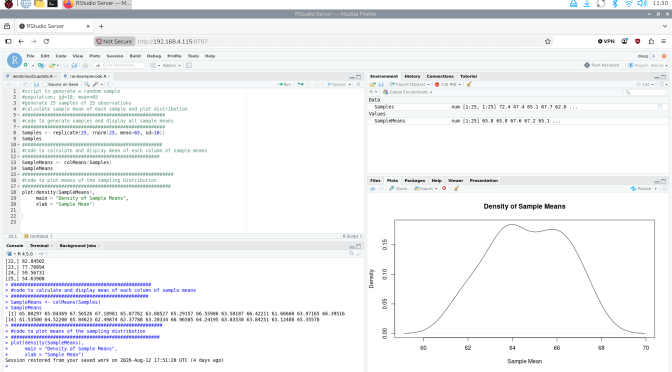
The screenshot shown below shows RStudio with the code from this article and the resulting output.

<Screenshot can be viewed in the PDF version of this document>

II. Using R on an Android Device

R and RStudio will not port directly to an Android based OS, but there are a few applications that will work with varying degrees of utility. I have a tablet that runs Android 16 and am using a free application, Rlytic,. Once installed from the Play Store users sign up with a username and password. When the program starts, a code entry console is displayed. Your code can be entered directly using the on-screen keyboard provided or can be loaded from your device file storage or cloud storage. The interface is easy to use. I have included a simple program example and some screenshots below.
Rlytic is free to use but is restricted to having only 2 programs active at a time. An unlimited version is available for purchase. I might also add that at the time of this writing Rlytic is running on R-base v.3 so users may run into some problems with more complex projects.

III. Using R on an iPhone

I currently use an iPhone 12 and was curious about any R applications that would work with it. I found an application called WebR which combines R-base 4.xxx with a text editor and browser interface. According to the program s author the application was designed for use by students in a classroom setting when learning statistics and/or R programming. It provides a highly mobile platform for Running R programs and quickly generates both text and graphics output. Once again, I will leave it to readers to engage the application s learning curve and will provide a simple example and screenshots below. The software is free and is available in the iPhone App Store.

IV. Sample Program: Raspberry Pi

The following code is a simple example of how R can be used to demonstrate the Central Limit Theorem in sampling from a population. The code uses the R-base rnorm function to generate randomly selected samples from a normally distributed population of values with a given population mean and standard deviation, finds the mean of each sample generated and graphs the sampling distribution. The code is shown below.

#population; sd=10; mean=65
#generate 25 samples of 25 observations
#calculate sample mean of each sample and plot distribution
###################################################
#code to generate samples and display all sample means
###################################################
Samples <- replicate(25, rnorm(25, mean=65, sd=10))
Samples #show the samples generated
##################################################
#code to calculate and display mean of each column of sample means
#################################################
SampleMeans <- colMeans(Samples)
SampleMeans #show the means of the samples generated
####################################################
#code to plot means of the sampling distribution
#####################################################
plot(density(SampleMeans),
main = “Density of Sample Means”,
xlab = “Sample Mean”)
The plot of the distribution of the sample means is shown below.

<Screenshot can be viewed in the PDF version of this document>

V. Sample Program: Rlytic
Here is the same code with the plot of the results for the Rlytic app on my Android 16 tablet. For brevity I have not included all the hashtag dialog from the RPi example. The screenshot and plot are shown.
#population; sd=10; mean=65
#generate 25 samples of 25 observations
#calculate sample mean of each sample and plot distribution
Samples <- replicate(25, rnorm(25, mean=65, sd=10))
#Samples
SampleMeans <- colMeans(Samples)
#SampleMeans
plot(density(SampleMeans),
main = “Density”,
xlab = Mean”)
The Rlytic Screen:

<Screenshot can be viewed in the PDF version of this document>

The Rlytic Plot: (Note Rlytic graphs are PDF format)

<Screenshot can be viewed in the PDF version of this document>

VI. Sample Program: WebR for iPhone
Here is a slightly modified version of the random sampling code entered into WebR on my iPhone 12.
x=rnorm(25, mean=65, sd=10)
plot(density(x))
Shown below is the resulting output. As in previous examples I did not print the output showing the randomly generated individual means.

<Screenshot can be viewed in the PDF version of this document>

I am still working on the next part of my tutorial on using wordcloud and related packages for the analysis of large, complex text files. Please look for my next post in the not-too-distant future.
D.M. Wiig
R Statistics and Programming
https://dmwiig.net

Visual Representation of Complex Data Using R: The tm and wordcloud Packages: Part One Revisited and Updated


I am uploading this “revision of the Revisited and updated” post in a plain text format to better facilliate the use of RSS feed readers to access the article. Links to the PDF version of this posting and the SOTU text file are at the bottom of the my previous post.

After a hiatus during which I retired from a teaching career I am returning to a project that I started nearly five years ago. I have published on this site many tutorials using R analysis to examine large data sets with many variables. My last post on this was part one of a project that involves large data sets composed of text data such as speeches. Virtually any collection of text can be processed using R and numerous R packages have been developed to generate various types of statistical analysis such word frequency counts and correlations among word frequencies. These statistics help enhance the information that is presented visually in the wordcloud graphic generated by the packages discussed in the Part One tutorial.

In this updated version of the Part One tutorial I will review the use of these tools using updated R packages and an analysis using text of the 2026 State of the Union Address. As indicated in Part One, full texts of State of the Union Addresses are available in several formats that can be downloaded. These cover Presidents from George W. Bush to the current term of Donald Trump, and can be found at https://www.govinfo.gov/features/state-of-the-union

There are other sources for SOTU texts but the government website allows quick selection of a file and one click to download the file. I simply save the selected file into a Windows Notepad text file. Make sure when you view the downloaded file that it is in an 80 column format and not formatted to fit a small screen such as a cellphone or tablet. I have found at least a couple of these files that are in the latter format and are not read correctly by the R functions presented in this paper.

The 2026 address was formatted originally in a small screen format. I found a wide-column transcript that I have used in this analysis. A link to the file is found on this website at the end of the article.

This section contains the updated R code that was presented in part one of this project. As indicated above, the resulting wordcloud is from the 2026 State of the Union. Additional code is presented in this section to calculate and print a word frequency table and to print a matrix of word association coefficients for the most used words.

Before diving into the code make sure that you have installed the latest version of the R console or an IDE such as RStudio. As I have stated earlier, I highly recommend the use of RStudio as a development environment and all of the projects presented on this website were coded and refined on this platform. As is the case with any IDE there is a learning curve, but if you are more than a casual programmer the learning process is well worth the effort. If you are using the R console and want to make sure all packages are up to date you can use the following code
#################################################################################script to access and install the newest version of the R console
###############################################################################
#the console should be updated from the Windows R console not from RStudio
#use the following code from the console
################################################################################
install.packages(“installr”) #download installer
library(installr) #move installer to library
updateR() #run the update; follow prompts as needed
################################################################################

The updated wordcloud code as shown below has been extensively commented as to the purpose of the sections within the program structure. For the sake of brevity I will not repeat the explanations contained in the original posting of this document. You can refer to that document on this website if necessary. I should also point out that you can copy all or parts of the code as presented here and paste it into the R console or RStudio code section. It should run properly. I tried to present the code in sections delimited by comments that allow segments to run individually for debugging purposes. As noted in the comments, make sure you change the table function argument section to point to the location of your downloaded text file. The complete code is seen below.


#NOTE:THIS SECTION HAS BEEN UPDATED WITH TRUMP SOTU 2026 DATA
#this is an updated version of Wordcloud1 that will include
#analysis and graphic representation of word counts and association coefficients
#for a single SOTU, Trump 2026
####################################################
#Load required packages
#####################################################
install.packages(“tm”) #processes data
install.packages(“wordcloud”) #creates visual plot
install.packages(“tidyverse”) #graphics utilities
install.packages(“readr”) #to load text files
install.packages(“RColorBrewer”) #for color graphics
#####################################################
#####################################################
#Load and view raw 2026 SOTU text file ‘sotu26.txt’
#Use RStudio Import Dataset tab or code below
#NOTE: BE SURE TO CHANGE THE read_table ARGUMENT TO
#POINT TO THE LOCATION OF THE FILE YOU ARE USING
#####################################################
library(readr)
statu26 <- read_table(“e:/dellfiles/sotu26.txt”, col_names = FALSE) #make sure this points to your file location!
#View(statu26)
####################################################
#Take raw text file statu26 and convert to corpus format named docs26
#####################################################
library(tm)
docs26 <- Corpus(VectorSource(statu26))
####################################################
#Clean punctuation, stopwords, white space
#Three passes create corpus vector source from original file
#A corpus is a collection of text
#One of the functions removes ‘stopwords’, words that are pre-defined
####################################################
library(tm)
library(wordcloud)
data(docs26)
docs26 <- tm_map(docs26, function(x)removeWords(x,stopwords()))
docs26 <- tm_map(docs26,removePunctuation) #remove punctuation
################################################################
#remove stopwords using with ‘en’ or ‘SMART’ criteria
docs26 <- tm_map(docs26,removeWords,stopwords(“SMART”))
###############################################################
docs26 <- tm_map(docs26,stripWhitespace) #remove white space
####################################################
#Cleaned corpus is now formatted into text document matrix
#Then frequency count done for each word in matrix
#dmat <-create matrix; dval <-sort; dframe <-count word frequencies
###################################################
docmat <- TermDocumentMatrix(docs26)
dmat <- as.matrix(docmat)
dval <- sort(rowSums(dmat),decreasing=TRUE)
dframe <- data.frame(word=names(dval),freq=dval)
####################################################
#Final step is to use wordcloud to generate graphics
#There are a number of options that can be set
#Use RColorBrewer to generate a color wordcloud
####################################################
library(RColorBrewer)
set.seed(1234) #use if random.color=TRUE
par(bg=”white”) #background color
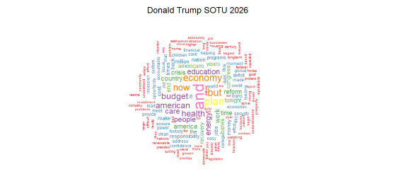
wordcloud(dframe$word,dframe$freq,colors=brewer.pal(8,”Set1″),random.order=FALSE,scale=c(2.75,0.35),min.freq=2,max.words=150,rot.per=0.35)
###################################################
####################################################
# Add a title above the plot
mtext(“Donald Trump SOTU 2026”, side = 3, line = 2, cex = 1.5)
##############################################################################
#this section contains code for printing word freq tables;
#word assoc analysis
#########################################################
#code to print 15 most used words with freq
####################################################
#for 2026 address
head(dframe,15)
######################################################
#code to find associations among specified terms
#drops assoc < .25
#initial setup formost frequent words; used between 10 and 25 times
#####################################################
#for 2026 address
findAssocs(docmat,terms = c(“and”,”but”,”budget”,”know”,”economy”,”health”,”plan”,”american”,”energy”,”people”,”care”),corlimit = .25)
######################################################


The output from the code will produce the wordcloud graphic display, a list of the most frequently used words in the document, and a matrix that displays association strengths equal to or greater than .25 for eleven of the most frequently used words in the document. A specific analysis of word frequencies and associations will be the topic of a future paper.

Shown below is the wordcloud graphic, the table of most frequently used words, and a portion of the association matrix generated by the code. I have only shown the portion of the matrix using the four most frequently used words.


Word Frequencies

word freq
and and 25
plan plan 16
but but 15
economy economy 14
now now 13
budget budget 12
health health 12
american american 12
education education 11
energy energy 11
people people 10
care care 10
country country 9
work work 9
america america 9


The association matrix:

$and
along already cmadam first now over second
0.85 0.85 0.85 0.85 0.85 0.85 0.85
speaking still thanks these third the this
0.85 0.85 0.85 0.85 0.85 0.79 0.73
for finally because there you its meet
0.71 0.64 0.50 0.44 0.44 0.41 0.29
bay career claims classroom commerce conscience earned
0.29 0.29 0.29 0.29 0.29 0.29 0.29
fallen ignore import industries ineffective layoffs marketbased
0.29 0.29 0.29 0.29 0.29 0.29 0.29
member message pad perseveres piles pride retooled
0.29 0.29 0.29 0.29 0.29 0.29 0.29
sacrifice succeed warera wealthy
0.29 0.29 0.29 0.29

$but
along already cmadam first over second
0.83 0.83 0.83 0.83 0.83 0.83
speaking still thanks these third now
0.83 0.83 0.83 0.83 0.83 0.81
the this for there finally because
0.81 0.65 0.64 0.64 0.53 0.43
you its agribusiness anger breaks cities
0.43 0.35 0.30 0.30 0.30 0.30
compete csomewhere lower messes pakistan percent
0.30 0.30 0.30 0.30 0.30 0.30
presidents pushed readying reality rebuilt set
0.30 0.30 0.30 0.30 0.30 0.30
transformation view
0.30 0.30

$plan
bank stand held full lose president
0.44 0.42 0.42 0.42 0.42 0.42
weakened builds challenge cmr intend preserve
0.42 0.41 0.41 0.41 0.41 0.41
progress proud respond tells creating cvice
0.41 0.41 0.41 0.41 0.41 0.41
deeds flow friends greensburg honest illusions
0.41 0.41 0.41 0.41 0.41 0.41
ive leonard outstanding prescription speak stopped
0.41 0.41 0.41 0.41 0.41 0.41
strain transform tysheoma boldly candidly doors
0.41 0.41 0.41 0.41 0.41 0.41
join men opinions recognizes showing stability
0.41 0.41 0.41 0.41 0.41 0.41
summit teachers team town save understand
0.41 0.41 0.41 0.41 0.35 0.34
asked recovery
0.30 0.28

$economy
assistance laughter abroad carry comforted costs
0.51 0.51 0.50 0.50 0.50 0.50
cunited cynical direct dramatically gains neighbors
0.50 0.50 0.50 0.50 0.50 0.50
oversight planet receive strategy taking teach
0.50 0.50 0.50 0.50 0.50 0.50
tornado troops auto industry energy act
0.50 0.50 0.37 0.37 0.32 0.30
held hold promise countries government ability
0.30 0.30 0.30 0.30 0.30 0.30
expanded build family social
0.30 0.30 0.30 0.30

In part two of this project I will expand the code to generate comparison clouds and associated statistics for two or more text files. Once again I will use State of the Union texts as the data for analysis. It is my hope that these R tutorials and examples have provided readers with some useful information and working models that can be adapted to their own research projects.

All R programming for this project was done using RStudio 2026.07.0+139 “Pacific Dogwood.”
This PDF document was produced using TeXstudio 4.9.5 (git 4.9.5)
Using Qt Version 6.11.0, compiled with Qt 6.11.0 R.
R, RStudio, and TeXstudio are free, open-source software.
Author: Douglas M. Wiig 7/31/2026
https://dmwiig.net

← Back

Thank you for your response. ✨

Visual Representation of Complex Data Using R: The tm and wordcloud Packages: Part One Revisited and Updated