An R tutorial by D. M. Wiig
This posting contains an embedded Word document. To view the document full screen click on the icon in the lower right hand corner of the embedded document.
An R tutorial by D. M. Wiig
This posting contains an embedded Word document. To view the document full screen click on the icon in the lower right hand corner of the embedded document.
An R tutorial by D. M. Wiig
This section gives examples of code to perform some of the most common elementary statistical procedures. All code segments assume that the package ‘car’ has been loaded and the file ‘Freedman’ has been loaded as the active dataset. Use the menu from the R console to load the ’car’ dataset or use the following command line to access the CRAN site list and packages:
install.packages()
Once the ’car’ package has been downloaded and installed use the following command to make it the active library.
require(car)
Load the ‘Freedman’ data file from the dataset ‘car’
data(Freedman, package="car")
List basic descriptives of the variables:
summary(Freedman)
Perform a correlation between two variables using Pearson, Kendall or Spearman’s correlation:
cor(filename[,c("var1","var2")], use="complete.obs", method="pearson")
cor(filename[,c("var1","var2")], use="complete.obs", method="spearman")
cor(filename[,c("var1","var2")], use="complete.obs", method="kendall")
Example:
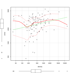
cor(Freedman[,c("crime","density")], use="complete.obs", method="pearson")
cor(Freedman[,c("crime","density")], use="complete.obs", method="kendall")
cor(Freedman[,c("crime","density")], use="complete.obs", method="spearman")
In the next post I will discuss basic code to produce multiple correlations and linear regression analysis. See other tutorials on this blog for more R code examples for basic statistical analysis.
R For Beginners: Some Simple R Code to Load a Data File and Produce a Histogram
A tutorial by D. M. Wiig
I have found that a good method for learning how to write R code is to examine complete code segments written to perform specific tasks and to modify these procedures to fit your specific needs. Trying to master R code in the abstract by reading a book or manual can be informative but is more often confusing. Observing what various code segments do by observing the results allows you to learn with hands-on additions and modifications as needed for your purposes.
In this document I have included a short video tutorial that discusses loading a dataset from the R library, examining the contents of the dataset and selecting one of the variables to examine using a basic histogram. I have included an annotated code chunk of the procedures discussed in the video.
The video appears below with the code segment following.
Here is the annotated code used in the video:
