I continue to complete work on my next post on using the R wordcloud package. As I normally do programming and wrting with my Lenovo desktop computer, I decided to experiment with installing R-base and RStudio on my Raspberry Pi Model 3B and tablet computer for those occasions when I desire to work while traveling. The Raspberry Pi is running the latest version of Debian Trixie along with the Raspberry Pi desktop. The tablet is using the latest version of Android 16. My first observation relates to the availability of R for these platforms.
I. Installing R-base and RStudio on Raspberry Pi3/B,4,5
R is available for a variety of UNIX, Windows, and MacOS systems. If you are running R on Windows, you are familiar with the 32- and 64-bit versions available for download and installation via an executable loader. While the R-base console has been available for the RPi platform, it has only been recently that the RStudio-server has been available for the ARM64 processor used in the RPi 3A/B, 4, and 5 models. I am currently using Debian Trixie 64-bit on my RPi 3/B. The R-base package is now available in Debian repositories so R can be installed via the RPi desktop menu rather than downloading binary builds or executable files.
For an RPi 3B or higher I would recommend the following:
-Make sure your microSD card is large enough. I am using a 32 GB card.
-Make sure your OS is up to date. Use the command line utility to run the following commands:
sudo apt update (respond to prompts that follow)
sudo apt full-upgrade (respond the prompts)
Depending on the model of RPi you are using, the memory card size and Debian version you are using this update could take quite some time.
Once the update is completed use the desktop menu to access the add/delete software option, search for the R package using r-base as the keyword and click on the appropriate icon to start the installation. When the installation is complete you should see the R icon in the desktop dropdown menu under the Programming or Science (or both) headings. The R-base console can now be run by clicking the menu icon, and R is now available for access by RStudio-server if it is installed.
Because the RPi uses an ARM processor, RStudio itself cannot be installed, but RStudio-server has been successfully ported to the platform. Additional information on R downloads can be found at the Posit web site RStudio IDE User Guide RStudio User Guide, and at the link RStudio Latest Builds. If you wish to install the RStudio-server from your RPi command line utility there are several steps, but the result is a working web-based interface with full RStudio-server build. Follow the steps listed below.
1. When installing new software run an update using:
sudo apt update
2. The port of RStudio-server we are installing was designed for the Ubuntu OS so install dependencies needed for Debian using:
sudo apt install gdebi-core libssl-dev libclang-dev
3. Get the build from the Posit Daily Builds library using
wget https://dl.dailies.rstudio.com/server/jammy/arm64/rstudio- server-2026.06.0-242-arm64.deb
4. Install the application using:
sudo gdebi rstudio-server-2026.06.0-242-arm64.deb
5. When the installation is complete use the system service command to start RStudio-server with:
sudo systemctl start rstudio-server (for the current bootup) and/or
sudo systemctl enable rstudio-server (start at all bootups)
6. Open the Chromium or Firefox web browser from the desktop menu and access the RStudio-server by entering the URL:
http://<RPi IP address on your network>:8787
In my case I would enter http://192.168.4.115:8787
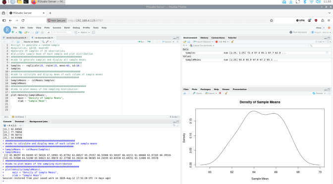
The screenshot shown below shows RStudio with the code from this article and the resulting output.
<Screenshot can be viewed in the PDF version of this document>
II. Using R on an Android Device
R and RStudio will not port directly to an Android based OS, but there are a few applications that will work with varying degrees of utility. I have a tablet that runs Android 16 and am using a free application, Rlytic,. Once installed from the Play Store users sign up with a username and password. When the program starts, a code entry console is displayed. Your code can be entered directly using the on-screen keyboard provided or can be loaded from your device file storage or cloud storage. The interface is easy to use. I have included a simple program example and some screenshots below.
Rlytic is free to use but is restricted to having only 2 programs active at a time. An unlimited version is available for purchase. I might also add that at the time of this writing Rlytic is running on R-base v.3 so users may run into some problems with more complex projects.
III. Using R on an iPhone
I currently use an iPhone 12 and was curious about any R applications that would work with it. I found an application called WebR which combines R-base 4.xxx with a text editor and browser interface. According to the program s author the application was designed for use by students in a classroom setting when learning statistics and/or R programming. It provides a highly mobile platform for Running R programs and quickly generates both text and graphics output. Once again, I will leave it to readers to engage the application s learning curve and will provide a simple example and screenshots below. The software is free and is available in the iPhone App Store.
IV. Sample Program: Raspberry Pi
The following code is a simple example of how R can be used to demonstrate the Central Limit Theorem in sampling from a population. The code uses the R-base rnorm function to generate randomly selected samples from a normally distributed population of values with a given population mean and standard deviation, finds the mean of each sample generated and graphs the sampling distribution. The code is shown below.
#population; sd=10; mean=65
#generate 25 samples of 25 observations
#calculate sample mean of each sample and plot distribution
###################################################
#code to generate samples and display all sample means
###################################################
Samples <- replicate(25, rnorm(25, mean=65, sd=10))
Samples #show the samples generated
##################################################
#code to calculate and display mean of each column of sample means
#################################################
SampleMeans <- colMeans(Samples)
SampleMeans #show the means of the samples generated
####################################################
#code to plot means of the sampling distribution
#####################################################
plot(density(SampleMeans),
main = “Density of Sample Means”,
xlab = “Sample Mean”)
The plot of the distribution of the sample means is shown below.
<Screenshot can be viewed in the PDF version of this document>
V. Sample Program: Rlytic
Here is the same code with the plot of the results for the Rlytic app on my Android 16 tablet. For brevity I have not included all the hashtag dialog from the RPi example. The screenshot and plot are shown.
#population; sd=10; mean=65
#generate 25 samples of 25 observations
#calculate sample mean of each sample and plot distribution
Samples <- replicate(25, rnorm(25, mean=65, sd=10))
#Samples
SampleMeans <- colMeans(Samples)
#SampleMeans
plot(density(SampleMeans),
main = “Density”,
xlab = Mean”)
The Rlytic Screen:
<Screenshot can be viewed in the PDF version of this document>
The Rlytic Plot: (Note Rlytic graphs are PDF format)
<Screenshot can be viewed in the PDF version of this document>
VI. Sample Program: WebR for iPhone
Here is a slightly modified version of the random sampling code entered into WebR on my iPhone 12.
x=rnorm(25, mean=65, sd=10)
plot(density(x))
Shown below is the resulting output. As in previous examples I did not print the output showing the randomly generated individual means.
<Screenshot can be viewed in the PDF version of this document>
I am still working on the next part of my tutorial on using wordcloud and related packages for the analysis of large, complex text files. Please look for my next post in the not-too-distant future.
D.M. Wiig
R Statistics and Programming
https://dmwiig.net