Tag Archives: r tutorial

Using R to Create Ternary Graphs


I am currently working on an updated posting of my tutorial
Ternary Diagrams Using R: An Example Using Election Outcomes.

The new tutorial will explore using ternary diagrams to track shifts in support for presidential candidates in the 2016 US presidential campaign.

Check back soon for the first installment!

Ternary Diagrams Using R: An Example Using Election Outcomes


Ternary Diagrams Using R:  An Example Using Election Outcomes

A tutorial by D. M. Wiig

In part one of this tutorial I discussed creating a ternary diagram using a simple data frame that contained five hypothetical cases. In this tutorial I will expand on that foundation by creating a more informative ternary diagram using live data.

A useful application of this package in social science research is creating a visual display of parliamentary election outcomes. Specifically we can use a ternary graph to examine the distribution of seats in the British House of Commons over a period of time. Since the UK uses a proportional system to allocate seats in the House of Commons there can be a variety of outcomes in any given national election.

Since 1945 general elections in the UK have produced a division of seats among the Labour, Conservative, and various minor parties. To demonstrate how this division of seats can be shown over time data was collected for all of the general elections from the years 1945 to 2015. These data show the percentage of the popular vote won by each party and the number of seats allocated to that party based on the vote division(retrieved from http://www.ukpolitical.info).  I have created a summary table of these results as follows:

Year   Con   Lab   LD+Other   SeatsCon   SeatsLab   SeatsOther

2015  36.9  30.4      32.7                331                232                 95

2010  36.1   29         34.9                 306               258                  85

2005  35.2   32.4    32.4                 355               198                  92

2001 40.7   31.7     27.6                 412               166                   81

1997 43.2  30.7     26.1                  418               165                   76

1992  42.3 35.2     23.5                   336              271                    44

1987  42.2 30.8     27                       375             229                    48

1983  42.4  27.6    26.9                    397             209                   27

1979  43.9 36.9    15.8                     339             268                    28

1974  39.2 35.8    21.8                   319             276                     39

1974  37.1 37.9    20.1                  301             296                     38

1970  46.4   43       8.6                   330             287                    19

1966  47.9 41.9     8.5                   363             253                     25

1964  44.1 53.4   11.2                  317             304                   22

1959  49.4  43.8    5.9                    365           258                    19

1955  49.7  46.4       0                     344            277                   18

1951  48    48.8        2.5                 321            295                   18

1950  46.1 43.5       9.1                315             297                   22

1945  47.8 39.8         1                  393            213                    57

The UK has a two party dominant system with a number of minor parties that regularly contest elections. As indicated above, a proportional representation method of allocating seats is used so these minor parties are able to gain some representation in the Commons. For readers interested in learning more about political parties in the UK there are a number of resources readily available at various online and other sources.

For purposes of this example I have added the popular vote of all minor parties together in the ‘LD+Other’ column, and the number of seats gained in the ‘SeatsOther’ column. By plotting the three variables ‘SeatsCon’, ‘SeatsLab’, and ‘SeatsOther’ by year on a ternary diagram we can visualize any changes in the mixture of seats won for the three groups. Before working through this tutorial make sure that you have the ggplot, ggplot2, and ggtern packages loaded into your R environment.

I originally created the table shown above using Excel and then imported it into R studio for analysis. If you are not using R studio you can enter the data via the R data editor as shown in the previous tutorial, or put the data into an Excel or LibreOffice spreadsheet and import it into R using the read.spss() function that I have discussed in earlier tutorials. You can also use any other method that you are familiar with to get the data into your R environment.

Once the data set is loaded use the following code to create the ternary diagram. Note that in this diagram we are using the base code as shown in the first tutorial with some additions that make the diagram easier to interpret such as the vector arrows and legend. The code segment is:

################################################### #create ternary plot using seats allocated by party for each election #uses enhanced formatting for easier interpretation #results of #ggtern function are placed in ‘plot for rendering ################################################### plot <- ggtern(data = ukvotedata, aes(x = SeatsCon, y = SeatsLab, z = SeatsOther)) +geom_point(aes(fill = Year), size = 4, shape = 21, color = “black”) + ggtitle(“Proportion of Seats Won 1945-2015”) + labs(fill = “Year”) + theme_rgbw() + theme(legend.position = c(0,1), legend.justification = c(0, 1)) ###################################################

To show the diagram simply use:

################################################### #now plot the diagram ################################################### plot ###################################################

The resulting ternary diagram is:

ukfinalplot

Each point on the graph represent the relative division of seats for each of the 19 elections in the table. The shading represents the year with the darkest being 1945 and the lightest 2015. The diagram clearly shows the trend toward more minor party representation and a move away from the two major parties over time. Indeed coalition governments resulted in several of the more recent elections due to the increase in minor party influence.

My purpose here is not to discuss UK politics but to show how ternary diagrams can be used in a social science application. With the many additions and extensions that are being added to the ggtern package it can be a very power device for graphical analysis.

Ternary Diagrams Using R: The ggtern Package


Ternary Diagrams Using R: The ggtern Package

A tutorial by Douglas M. Wiig

There are a number of very useful and popular graphics packages available for R such as lattice, ggplot, ggplot2 and others. Some of these offer general purpose graphics capabilities and others are more specialized. A recently developed extension to the ggplot2 package is ggtern. This package is essentially a wrapper for a number of functions that can be used to create a variety of ternary diagrams. Ternary diagrams are useful when analyzing the relationship among three factors or elements. A ternary diagram essentially represents the proportions of three related factors in two-dimensional space.

Before running the script in this tutorial make sure that the packages ggplot, ggplot2, and ggtern are loaded into your R environment. A basic graph can be easily constructed. I will the use theoretical quantities Xa , Xb , and Xc to demonstrate a basic ternary diagram. In this simple example I will create a sample of n=5 by entering the data from the keyboard into a data frame ‘sampfile.’ To invoke the editor use the following code:

################################################### #create a sample file of n=5 ################################################### sampfile <-data.frame(Xa=numeric(0),Xb=numeric(0),Xc=numeric(0)) sampfile <-edit(sampfile) ###################################################

This will open up a data entry sheet with three columns labeled Xa, Xb, and Xc. The number that are entered do not matter for purposes of this illustration. The table I entered is as follows:
Xa      Xb        Xc

1 100  135     250

2 90    122     210

3 98    144    256

4 100    97      89

5  90     75      89

To produce a very basic ternary diagram with the above data set use the command:

################################################## #do basic graph with sample data ################################################## ggtern(data=sampfile,aes(x=Xa,y=Xb, z=Xc))+geom_point() ##################################################

This produces the graph seen below:

ggterm[;ptbasoc
As can be seen the triangular representation of the dimensions Xa →Xb, Xc → Xa and Xb →Xc allow each case to be represented as a single point located relative to each of the three vectors. There are a large number of additions, modifications and tweaks that can be done to this basic pattern.

In the next tutorial I will discuss generating a more elaborate ternary diagram using election outcome data from British general elections. For more information about the ggtern package see the CRAN documentation and information as well as the web site http://www.ggtern.com for all of the latest news and developments.

Using R: Random Sample Selection and One-Way ANOVA


A tutorial by Douglas M. Wiig

In the previous tutorial we looked at the hypothesis that one’s outlook on life is influenced by the amount of education attained. Using the GSS 2014 data file we looked at the education variable ‘educ’, and the outlook on life variable ‘life’, a measure of outlook on life as ‘DULL’, ‘ROUTINE’, or ‘EXCITING.’ We selected a subset for each response category and found that there appeared to be
differences among the mean level of education measured in years for each of the categories of outlook on life. To further examine this we will first randomly select a sample from the data file, look at the
mean education for each category of outlook on life, and evaluate the means using simple one-way ANOVA.

To randomly select a sample from a population of values we can use the sample() function. There are a number of options and variations of the function that are beyond the scope of this tutorial. Since the
variable ‘educ’ is measured in years we can use the sample.int() function which is designed for use with integer values. The general format of the function is:

sample.int(n, size = n, replace = FALSE)

where: n = the size of population the sample is from
size = the size of the sample
replace = FALSE if sampling without replacement; TRUE if sampling with replacement

For this example I will select a sample of n=500 without replacement from the data file containing a total of 2538 cases. The sample data is loaded into a data matrix as it is selected. This will be
accomplished in two steps. In the first step we will load the sample.int() function with the values to use for selecting the sample and put the vector in ‘randsamp2. The code is:

randsamp2 <- sample.int(2538, size=500, replace=FALSE)

To select the sample make sure that make sure that the GSS2014 data file is loaded into the R environment. I previously loaded the data file into a data frame ‘gss14.’  To select the sample and load
it into a data frame ‘randgss2’ the code is:

randgss2 <- gss14[randsamp2,]

Once the sample has been generated we can look at the mean years of education for each of the three responses for outlook on life. We do this by selecting a subset for each response. Use the following
code:

###################################################
#look at educ means by life by selecting 3 subsets from randgss2
###################################################
life12 <- subset(randgss2, life == “DULL”, select=educ)
life22 <- subset(randgss2, life == “ROUTINE”, select=educ)
life32 <- subset(randgss2, life == “EXCITING”, select=educ)

Now run summary statistics for each subset to look at the means:

summary(life12)
summary(life22)
summary(life32)

We can now see that the means are as follows:

life12 = 13.0
life22 = 13.29
life 32 = 14.51

and we can generate a summary visual of the differences among the three subsets by doing a simple boxplot using:

###################################################
# do boxplots of the subsets to visualize differences
#boxplot using educ and life variables from the ‘randgss2’ data #frame
###################################################
boxplot(randgss2$educ ~ randgss2$life, main=”Education and View on Life n = 500″, xlab=”View of Life”,ylab=”Years of Education”)

The following graph will result:

Rplotrandgss2

As can be seen above there does appear to be a difference among these means, particularly for those who see life as ‘DULL.’ To see if these differences are significant an ANOVA will be run using the
simple one way ANOVA function aov(). The basic function is:
aov(formula, data = NULL)For our example we use:

model2 <- aov(educ ~ life, data=randgss2)

which analyzes the mean education by category of outlook on life using the randgss2 sample of n=500. The results are stored in ‘model2.’ The output from this operation is shown using the summary() function. This produces the following output:

summary(model2)

Df Sum Sq Mean Sq F value Pr(>F) life
2  171.5    85.77     10.42 4.08e-05 ***
Residuals  332     2732.2  8.23

Signif. codes: 0 ‘***’ 0.001 ‘**’ 0.01 ‘*’ 0.05 ‘.’ 0.1 ‘ ’ 1
165 observations deleted due to missingness

This output shows that at least one of the means differs significantly from the others. To test this difference further we can use a pair-wise comparison of means to see which means differ significantly
from each other. There are several options available. We will use a basic Tukey HSD comparison. This is accomplished using:

##################################################
#run HSD on sample
TukeyHSD(model2)
##################################################

producing the following output:

Tukey multiple comparisons of means
95% family-wise confidence level

Fit: aov(formula = educ ~ life, data = randgss2, projections = TRUE)

$life                               diff                     lwr                upr                    p adj
ROUTINE-EXCITING -1.074404 -1.833686 -0.31512199  .0027590
DULL-EXCITING          -2.729412 -4.447386 -1.01143754  .0006325
DULL-ROUTINE           -1.655008 -3.384551 0.07453525 00640910

By looking at the p value for each comparison it can be seen that both the ROUTINE-EXCITING and DULL-EXCITING means differ significantly at p ≤ .05

I might point out that if a researcher was using the GSS 2014 data file as we used here there would need to be more data preparation prior to running any analysis. For example, there is a fair amount of
missing data as indicated by NA in the raw data file. The missing data would need to be handled in some way. R has numerous functions and packages that can assist in resolving missing data issues of
various types, but a discussion of these is a subject for a future tutorial.
8/7/15                   Douglas M. Wiig                    http://dmwiig.net

Tutorial: Using R to Analyze NORC GSS Social Science Data, Part Six, R and ANOVA


Tutorial: Using R to Analyze NORC GSS Social Science Data, Part Six, R and ANOVA

A tutorial by Douglas M. Wiig

As discussed in previous segments of this tutorial, for anyone interested in researching social science questions there is a wealth of survey data available through the National Opinion Research Center (NORC) and its associated research universities. The Center has been conducting a national survey each year since 1972 and has compiled a massive database of data from these surveys. Most if not all of these data files can be accessed and downloaded without charge. I have been working with the 2014 edition of the data and for all part of this tutorial will use the GSS2014 data file that is available for download on the Center’s web site. (See the NORC main website at http://www.norc.org/Research/Projects/Pages/general-social-survey.aspx and at http://www3.norc.org/GSS+Website ).

Accessing and loading the NORC GSS2014 data set was discussed in part one of this tutorial. Refer to it if you need specific information on downloading the data set in STATA or SPSS format.  In this segment we will use the subset function to select a desired set of cases from all of the cases in the data file that meet certain criteria.  As indicated in my previous tutorial the GSS2014 data set contains a
total of 2588 cases and 866 variables.

Before starting this segment of the tutorial be sure that the foreign
package is installed and loaded into your R session. As I have indicated in previous tutorials, use of an IDE such as R Studio greatly facilitates entering and debugging R code when doing research such as is discussed in my tutorials.  

Import the GSS 2014 data file in SPSS format and load it into the data frame ‘gss14’ using:
#########################################################import  GSS2014 file in SPSS .sav format
#uses foreign package
########################################################require(foreign)
gss14<- read.spss("/path to your location/GSS2014.sav",                      use.value.labels=TRUE,max.value.labels=Inf, to.data.frame=TRUE)
#################################################

In this tutorial the analysis of this sample will focus on examining the hypothesis “An individual’s outlook on life is influenced by the amount of education the person has attained.” The GSS variables ‘educ’, education in number of years and ‘life’, whether the respondent rated life DULL, ROUTINE, or EXCITING. A simple approach to testing this hypothesis is to compare mean levels of education for each of the three categories of response. I will do this analysis in two stages. In the first stage I will use techniques discussed in a previous tutorial to select a subset of each response category and display the mean education level for each of the three categories.

The three subsets life1, life2, and life3 are generated using the following code:

###################################################
# create 3 subsets from gss14 view on life by years of education
##################################################

life1 <- subset(gss14, life == “DULL”, select=educ)

life2 <- subset(gss14, life ==”ROUTINE”, select=educ)

life3 <- subset(gss14, life == “EXCITING”, select=educ)

###################################################

#The three means of the subsets are displayed using the code:

# run summary statistics for each subgroup

##################################################

summary(life1)

summary(life2)

summary(life3)

###################################################

resulting the following output:
educ
Min. : 0.00
1st Qu.:10.00
Median :12.00
Mean :11.78
3rd Qu.:13.00
Max. :20.00

summary(life2)
educ
Min. : 0.00
1st Qu.:12.00
Median :13.00
Mean :13.22
3rd Qu.:16.00
Max. :20.00
NA’s :1

summary(life3)
educ
Min. : 2.00
1st Qu.:12.00
Median :14.00
Mean :14.31
3rd Qu.:16.00
Max. :20.00

As is seen above there does appear to be a difference among mean years of education and the corresponding outlook on life. In order to examine whether or not these observed differences are not due to chance a simple one-way Analysis of Variance can be generated.

In the next tutorial I will discuss performing the ANOVA and using pair-wise comparisons to determine which if any means are different.

R Tutorial: Using R to Analyze the NORC GSS2014 Database, Selecting Subsets and Comparing Means Using Student’s t Test


R Tutorial Part Three: Selecting Subsets and Comparing Means Using an Independent Sample t Test

A tutorial by Douglas M. Wiig

As discussed in previous segments of this tutorial, for anyone interested in researching social science questions there is a wealth of survey data available through the National Opinion Research Center (NORC) and its associated research universities. The Center has been conducting a national survey each year since 1972 and has compiled a massive database of data from these surveys. Most if not all of these data files can be accessed and downloaded without charge. I have been working with the 2014 edition of the data and for all part of this tutorial will use the GSS2014 data file that is available for download on the Center’s web site. (See the NORC main website at http://www.norc.org/Research/Projects/Pages/general-social-survey.aspx and at http://www3.norc.org/GSS+Website ).

Accessing and loading the NORC GSS2014 data set was discussed in part one of this tutorial. Refer to it if you need specific information on downloading the data set in STATA or SPSS format.  In this segment we will use the subset function to select a desired set of cases from all of the cases in the data file that meet certain criteria.  As indicated in my previous tutorial the GSS2014 data set contains a total of 2588 cases and 866 variables.
Before starting this segment of the tutorial be sure that the foreign package is installed and loaded into your R session.  Import the GSS 2014 data file and load it into the data frame ‘Dataset’ using:

########################################################
#import GSS2014 file in SPSS .sav format
#uses foreign package
########################################################
require(foreign)
Dataset <- read.spss("/path to your location/GSS2014.sav", 
                     use.value.labels=TRUE, max.value.labels=Inf, to.data.frame=TRUE)

###########################################################

In the previous segment of this tutorial we started to investigate whether or not an individual’s education had an effect on their response to a NORC survey item dealing with abortion. The item asked respondents to either ‘AGREE’ or ‘DISAGREE’ with the statement ‘A women should be allowed to obtain an abortion under any circumstances.’ We selected a subset of all of the respondents who answered ‘AGREE’ and a second subset of all the respondents who answered ‘DISAGREE’ using the following code:

##############################################

#select subset from Dataset and write to data frame SS1

###################################################
SS1 <- subset(Dataset, abany == "YES", select=educ)

View(SS1)

#######################################################

######################################################
#select subset from Dataset and write to data frame SS2
######################################################
SS2 <- subset(Dataset, abany == "NO", select=educ)
View(SS2)

A mean number of years of education can be calculated for each of the subsets using the following:

#calculate descriptive statistics for SS1 and SS2

####################################################

summary(SS1)

summary(SS2)

####################################################

Output from the above for SS1 is:

> summary(SS1)

educ

Min. : 0.0

1st Qu.:12.0

Median :15.0

Mean :14.6

3rd Qu.:16.0

Max. :20.0

Output for SS2 is:

> summary(SS2)

educ

Min. : 0.00

1st Qu.:12.00

Median :12.00

Mean :12.93

3rd Qu.:15.00

Max. :20.00

NA’s :1

As seen above there is a difference in mean years of education for the two subsets. We can use a two independent sample t test to determine whether or not the difference is large enough to not be due to chance.

In this tutorial I will use the Student’s t test function t.test that is found in the stats package. The function is used in the following form:

t.test =(x,y, alternative = c(“two.sided”, “less”, “greater”), mu=0, paired = FALSE, var.equal = FALSE, conf.level = .95)

where x and y = numeric vectors of data values

alternative = specification of a one-tailed or two-tailed test

mu = 0 specification that true difference between means is zero

paired = FALSE specification of a two independent sample test; if TRUE a paired samples test will be used

var.equal = specification of equal variances of the two samples; if TRUE the pooled variance is used otherwise a Welsh approximation of degrees of freedom is used

conf.level = confidence level of the interval

For further information see the documentation in CRAN help files for the function t.test().

Using the vectors selected from the dataset SS1, and SS2 the t test is performed using:

###########################################################

#perform a t test to compare sample means

#########################################################

t.test(SS1,SS2, alternative = c(“two.sided”), mu=0, paired=FALSE, var.equal = TRUE, conf.level = .95)

###########################################################

Resulting in output of:

        Two Sample t-test

data:  SS1 and SS2 
t = 11.1356, df = 1650, p-value < 2.2e-16
alternative hypothesis: true difference in means is not equal to 0 
95 percent confidence interval:
 1.369673 1.955333 
sample estimates:
mean of x mean of y 
 14.59517  12.93267 

We can see that the difference between the mean years of education for the ‘YES’ and the ‘NO’ samples is significant at an alpha level of p=.05. Subsets can also be used to compare means involving more than two samples and using simple one-way Analysis of Variance. This will be covered in the next part of the tutorial.

R Tutorial: Using the NORC GSS2014 Data File, Creating and Using Subsets


R Tutorial:  Using the NORC GSS2014 data file, creating and using subsets

By Douglas M. Wiig

As discussed in the first part of this tutorial, for anyone interested in researching social science questions there is a wealth of survey data available through the National Opinion Research Center (NORC) and its associated research universities. The Center has been conducting a national survey each year since 1972 and has compiled a massive database of data from these surveys. Most if not all of these data files can be accessed and downloaded without charge. I have been working with the 2014 edition of the data and for all part of this tutorial will use the GSS2014 data file that is available for download on the Center’s web site. (See the NORC main website at http://www.norc.org/Research/Projects/Pages/general-social-survey.aspx and at http://www3.norc.org/GSS+Website ).

Accessing and loading the NORC GSS2014 data set was discussed in part one of this tutorial. Refer to it if you need specific information on downloading the data set in STATA or SPSS format.  In this segment we will  use the subset function to select a desired set of cases from all of the cases in the data file that meet certain criteria.  As indicated in my previous tutorial the GSS2014 data set contains a total of 2588 cases and 866 variables.

One of the areas surveyed by NORC each year deals with attitudes toward abortion. One of the questions simply asks respondents if they '...approve of abortion under any circumstances.'  The response is either YES or NO to this question.  Let's assume a researcher is interested in investigating whether or not education has an effect on how the respondent answers the question.

To look at this hypothesis we can use the abortion attitude variable mentioned above, 'abany', and an education variable 'educ' which measures education as the actual number of years of education.  Twelve years of education would be a high school graduate for example, and 16 years would be a college graduate.  We can select a subset of all respondents who indicated 'YES' on the survey question and then generate a mean years of education for this subset.  We can then select a subset of all respondents who indicated 'NO' on the question and calculate a mean years of education for the second subset.

Before starting this code segment be sure that the foreign package is installed and loaded into your R session.  Import the GSS 2014 data file and load it into the data frame ‘Dataset’ using:

########################################################
#import GSS2014 file in SPSS .sav format
#uses foreign package
########################################################
require(foreign)
Dataset <- read.spss("/path to your location/GSS2014.sav", 
                     use.value.labels=TRUE, max.value.labels=Inf, to.data.frame=TRUE)
########################################################

Once the GSS2014 file is loaded use the subset function to select your first subset of respondents who answered the 'abany' question with and 'YES response.  Use the following code to select the subset and store it in a data frame 'SS1':

####################################################
#select subset from Dataset and write to data frame SS1
####################################################
SS1 <- subset(Dataset, abany == "YES", select=educ)
View(SS1)
####################################################

Now select a second subset of respondents who answered the 'abany' question with a 'NO' response. Use the following code to select the subset and store in a data frame 'SS2':

######################################################
#select subset from Dataset and write to data frame SS2
######################################################
SS2 <- subset(Dataset, abany == "NO", select=educ)
View(SS2)
######################################################

In using the subset function as seen above the name of the data set is specified, the criteria for selecting rows is given, and the variables to select from each row specified.  If no 'select' option is given all variables will be shown for the selected row.

Using the View command to examine each subset shows the years of education for each of the 746 respondents who answered ‘YES’ and each of the 907 respondents who answered ‘NO.’ Since the variable ‘educ’ is measured as ratio level numeric data we can calculate a mean and standard deviation for each subset and perform both graphical and statistical analysis of any observed difference between the two means. This will be the subject of the next installment of the tutorial.

R Tutorial: Using R with NORC GSS Data Part Two, Generating Simple Tables and Using Subsets


A tutorial by Douglas M. Wiig

Part one of the tutorial  centered on importing NORC GSS data in STATA or SPSS formats in an R data frame. For illustration I used the GSS2014 survey data set that consists of 2538 cases and 866 variables. If a researcher wishes to generate some simple cross tabulations the R CrossTable function is very useful.

The CrossTable function is part of the gmodels package, so before running scripts in this tutorial make sure you have installed and loaded gmodels from your favorite CRAN mirror site. As discussed in part one of the tutorial load the GSS2014 dataset into the global environment using:

>require(foreign)

>Dataset <- read.spss(“E:/research/Documents/GSS2014.sav”,

use.value.labels=TRUE, max.value.labels=Inf, to.data.frame=TRUE)

The CrossTable function allows a basic cross tabulation to be performed and includes a large number of options that can be incorporated into the table. The basic structure is as follows:

Usage

CrossTable(x, y, digits=3, max.width = 5, expected=FALSE, prop.r=TRUE, prop.c=TRUE,

prop.t=TRUE, prop.chisq=TRUE, chisq = FALSE, fisher=FALSE, mcnemar=FALSE,

resid=FALSE, sresid=FALSE, asresid=FALSE,

missing.include=FALSE,

format=c(“SAS”,”SPSS”), dnn = NULL, …)

Arguments

x A vector or a matrix. If y is specified, x must be a vector

y A vector in a matrix or a dataframe

digits Number of digits after the decimal point for cell proportions

max.width In the case of a 1 x n table, the default will be to print the output horizontally.

If the number of columns exceeds max.width, the table will be wrapped for

each successive increment of max.width columns. If you want a single column

vertical table, set max.width to 1

expected If TRUE, chisq will be set to TRUE and expected cell counts from the _2 will be

included

prop.r If TRUE, row proportions will be included

prop.c If TRUE, column proportions will be included

prop.t If TRUE, table proportions will be included

prop.chisq If TRUE, chi-square contribution of each cell will be included

chisq If TRUE, the results of a chi-square test will be included

fisher If TRUE, the results of a Fisher Exact test will be included

mcnemar If TRUE, the results of a McNemar test will be included

resid If TRUE, residual (Pearson) will be included

sresid If TRUE, standardized residual will be included

asresid If TRUE, adjusted standardized residual will be included

missing.include

If TRUE, then remove any unused factor levels

format Either SAS (default) or SPSS, depending on the type of output desired.

dnn the names to be given to the dimensions in the result (the dimnames names).

optional arguments

(Gregory Warnes, maintainer, Package ‘Gmodels’ February, 2015. http://cran.r-project.org/src/contrib/PACKAGES.html)

In this tutorial I will create a  table to examine the relationship between income and education using the variables ‘degree’ and ‘income6’ from the GSS dataset. Both are categorical factors. To simplify the resulting table only actual frequencies will be reported and the ‘chisq’ option will be used to generate a chi-squared test. The format used will be set to SPSS. Use the following statement:

>Generate a cross table of frequencies with chisq reported

>CrossTable(Dataset$”incom16″,Dataset$”degree”, chisq=TRUE, format=c(“SPSS”),prop.r=FALSE, prop.c=FALSE, prop.t=FALSE, prop.chisq=FALSE)

>

In the above code, the row variable is income the appropriate column of the dataset is selected with the ‘Dataset$”incom16” statement. The column variable for the table is education and the appropriate column of the dataset is selected with the ‘Dataset$”degree” statement. The various cell proportions must be set to ‘FALSE’ as they are defaulted to ‘True.’

When you run the above script the table will be generated in SPSS format on the screen.  I will not reproduce the table here because of formatting problems of fitting the table into the blog format.

In part three of this turorial I will discuss generating subsets of the GSS data file and using subsets for statistical analyses such as t tests and ANOVA.


Tutorial: Using R to Analyze GSS2014 Social Science Data, Part One: Importing the Database in SPSS or STATA Format


For anyone interested in researching social science questions there is a wealth of survey data available through the National Opinion Research Center (NORC) and its associated research universities. The Center has been conducting a national survey each year since 1972 and has compiled a massive database of data from these surveys. Most if not all of these data files can be accessed and downloaded without charge. I have been working with the 2014 edition of the data and for this tutorial will use the GSS2014 data file that is available for download on the Center’s web site. ( See the NORC main website at http://www.norc.org/Research/Projects/Pages/general-social-survey.aspx and at http://www3.norc.org/GSS+Website ).

As noted above the datasets that are available for download are available in both SPSS format and STATA format. To work with either of these formats using R it is necessary to read the file into a data frame using one of a couple of different packages. The first option I will discuss uses the Hmisc package. The second option I will discuss uses the foreign package. Install both of these packages from your favorite CRAN mirror site before starting the code in this tutorial.

For this tutorial I am using the one year release file GSS2014. This file contains 2538 cases and 866 variables. Download the file   from the web site listed above in both SPSS and STATA formats. Use the following code to load the Hmisc package into your R global environment:

                >require(Hmisc)

Now load the GSS2014.sav SPSS version from your storage device using the following line of code. I am using the filename GSS2014 for my data file and loading the file into the data frame ‘gss14’:

>#load the GSS data file in SPSS format

                >put data into data frame ‘gss14’

                gss14 <- spss.get(F:/research/Documents/GSS2014.sav”,                     use.value.labels=TRUE)

                >

To view the data that was loaded use the command:

>View(gss14)

This will produce a spreadsheet-like matrix of rows and columns containing the data. To load the data file in STATA format download the STATA version of the file from the NORC web site a discussed above. My STATA file is also named GSS2014, but with the STATA .dta extension. Load the file into a data frame using:

>load STATA format file into data frame ‘Dataset2’

                >Datatset2 <- read.dta(“F:/resarch/Documents/GSS2014.dta”)

               >

Once again, you can view the data frame loaded using the command:

>View(dataset2)

Both the STATA and SPSS formats of the data set can also be loaded into R using the foreign package. The procedure is the same for both SPSS and STATA

>load SPSS version

                >require(foreign)

                >Dataset <- read.spss(“F:/research/Documents/GSS2014.sav”,   use.value.labels=TRUE)

 >load STATA version into data frame ‘Dataset3’

>Dataset3 <- read.dta(“E:/research/Documents/GSS2014.dta”)

Use the ‘View()’ command to view the data frame.

In part two I will discuss some techniques using R to create and analyze subsets of the GSS2014 data file.


Using R for Nonparametric Analysis, The Kruskal-Wallis Test Part Four: R Script and Some Notes on IDE’s


Using R for Nonparametric Analysis, The Kruskal-Wallis Test: R Script and Some Notes on IDE’s


A tutorial by Douglas M. Wiig


In the previous three parts of this tutorial I discussed using R to enter a data set and perform a nonparametric Kruska-Wallis test for ranked means. In this final part the commented script that was used in the first three parts is listed. 


If you are going to use R for the majority of your statistical analysis it is highly advisable that you investigate some of the IDE’s (Integrated Development Environments) that are available to assist in coding and debugging R script and creating R packages for personal use or distribution. I think one of the easiest to use is R Studio. R Studio is available in both free open source and commercial versions and can be downloaded at http://www.rstudio.com    There are versions available for Windows, various Linux distributions, and Mac OS.

The R studio console provides a number of useful tools that facilitate coding. The screen is divided into four sections with one section providing a code editor that features syntax highlighting, code completion and many other features such as line or block code execution. Another window contains R and all displays output, error messages and warnings when code is executed from the editor. A third window displays all of the current environmental variables that are active and can also show all currently loaded R packages. A fourth window can show graphic output from executed code, can be used to manage, download and install R packages, and can be used to access the CRAN database of online help. There are other useful tools that are too numerous to discuss here.


Another program that is worth looking at is RKWard which combines an IDE with a graphics GUI for R statistical analysis. Information and downloads for RKWard can be found at https://rkward.kde.org. This program is also free and open source and can be run on a Windows platform, Mac OS, or various distributions of Linux. The program has been optimized for Linux. A discussion of these IDE’s is beyond the scope of this posting.


Shown below is the commented R script for all three parts of the Kruskal-Wallis tutorial. For ease of reading code portions are shown in bold print.


#packages that must be present in the global environment before running these scripts


#stats; graphics; grDevices; utils; datasets; methods; base


#


#code to enter data using the data editor


#KW data entry, define file kruskal as a data frame


kruskal <-data.frame()


#invoke the data editor


kruskal <-edit(kruskal)


#define group as containing 3 factors; tell R which data column goes with which factor


group <- factor(1,2,3)


#alternative data entry method


#Define factor Group as containing three categories


Group <- c(1,1,1,1,1,2,2,2,2,2,3,3,3,3)


#create a vector defined as authscore and enter values


authscore <- c(96,128,83,61,101,82,121,132,135,109,115,149,166,147)


#create data frame kruskal matching each group factor to individual scores


kruskal <- data.frame(Group, authscore)


#use the following line to look at the structure of the data frame created


str(kruskal)


#run the basic Kruskal-Wallis test


#


kruskal.test(authscore ~ Group, data=kruskal)


#


#the following code is used to conduct a post-hoc comparison of the ranked means


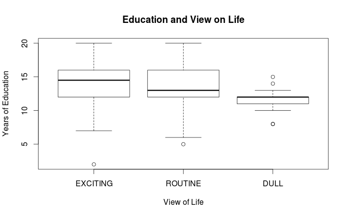
#it is useful to first do a simple boxplot for a visual comparison


#Use this script to save the boxplot graphic to a .png data file


#save output in pdf file authplot


#send output to screen and file


sink()


authplot <- boxplot(authscore ~ Group, data=kruskal, main=”Group Comparison”, ylab=”authscore”)


#save .png file


png(“authplot.png”)


#now return all output to console


dev.off()


#


#make sure that the package PMCMR is loaded before running the following script


library(PMCMR)


#use the ‘with’ function to pass the data from the kruskal data frame to the post hoc


#test script; specify the Tukey HSD method for determining significance of each


# pair of comparisions


#


with(kruskal, {


posthoc.kruskal.nemenyi.test(authscore, Group, “Tukey”)


})


#


#NOTE: if using a version of R < 3.xx then use the package pgirmess instead of PMCMR


#


#the following lines show the post hoc analysis using the pgirmess package


#note the function kuskalmc is used for the comparisons


library(pgirmess)


authscore <- c(96,128,83,61,101,82,121,132,135,109,115,149,166,147)


Group <- c(1,1,1,1,1,2,2,2,2,2,3,3,3,3)


kruskalmc(authscore ~ Group, probs=.05, cont=NULL)


#