A tutorial by Douglas M. Wiig

In the previous tutorial we looked at the hypothesis that one’s outlook on life is influenced by the amount of education attained. Using the GSS 2014 data file we looked at the education variable ‘educ’, and the outlook on life variable ‘life’, a measure of outlook on life as ‘DULL’, ‘ROUTINE’, or ‘EXCITING.’ We selected a subset for each response category and found that there appeared to be
differences among the mean level of education measured in years for each of the categories of outlook on life. To further examine this we will first randomly select a sample from the data file, look at the
mean education for each category of outlook on life, and evaluate the means using simple one-way ANOVA.

To randomly select a sample from a population of values we can use the sample() function. There are a number of options and variations of the function that are beyond the scope of this tutorial. Since the
variable ‘educ’ is measured in years we can use the sample.int() function which is designed for use with integer values. The general format of the function is:

sample.int(n, size = n, replace = FALSE)

where: n = the size of population the sample is from
size = the size of the sample
replace = FALSE if sampling without replacement; TRUE if sampling with replacement

For this example I will select a sample of n=500 without replacement from the data file containing a total of 2538 cases. The sample data is loaded into a data matrix as it is selected. This will be
accomplished in two steps. In the first step we will load the sample.int() function with the values to use for selecting the sample and put the vector in ‘randsamp2. The code is:

randsamp2 <- sample.int(2538, size=500, replace=FALSE)

To select the sample make sure that make sure that the GSS2014 data file is loaded into the R environment. I previously loaded the data file into a data frame ‘gss14.’  To select the sample and load
it into a data frame ‘randgss2’ the code is:

randgss2 <- gss14[randsamp2,]

Once the sample has been generated we can look at the mean years of education for each of the three responses for outlook on life. We do this by selecting a subset for each response. Use the following
code:

###################################################
#look at educ means by life by selecting 3 subsets from randgss2
###################################################
life12 <- subset(randgss2, life == “DULL”, select=educ)
life22 <- subset(randgss2, life == “ROUTINE”, select=educ)
life32 <- subset(randgss2, life == “EXCITING”, select=educ)

Now run summary statistics for each subset to look at the means:

summary(life12)
summary(life22)
summary(life32)

We can now see that the means are as follows:

life12 = 13.0
life22 = 13.29
life 32 = 14.51

and we can generate a summary visual of the differences among the three subsets by doing a simple boxplot using:

###################################################
# do boxplots of the subsets to visualize differences
#boxplot using educ and life variables from the ‘randgss2’ data #frame
###################################################
boxplot(randgss2$educ ~ randgss2$life, main=”Education and View on Life n = 500″, xlab=”View of Life”,ylab=”Years of Education”)

The following graph will result:

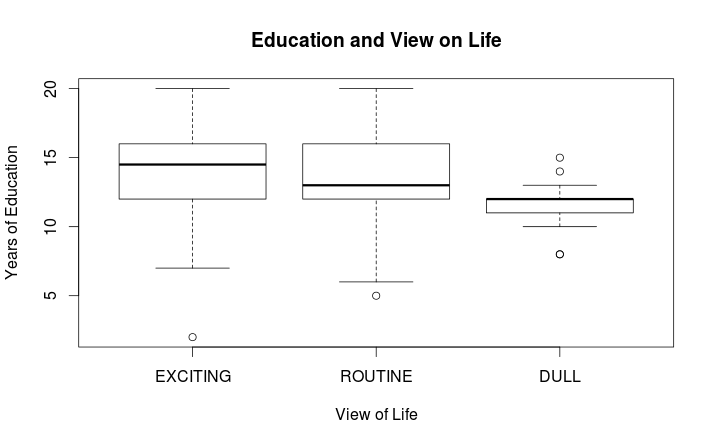
As can be seen above there does appear to be a difference among these means, particularly for those who see life as ‘DULL.’ To see if these differences are significant an ANOVA will be run using the
simple one way ANOVA function aov(). The basic function is:
aov(formula, data = NULL)For our example we use:

model2 <- aov(educ ~ life, data=randgss2)

which analyzes the mean education by category of outlook on life using the randgss2 sample of n=500. The results are stored in ‘model2.’ The output from this operation is shown using the summary() function. This produces the following output:

summary(model2)

Df Sum Sq Mean Sq F value Pr(>F) life
2  171.5    85.77     10.42 4.08e-05 ***
Residuals  332     2732.2  8.23
—
Signif. codes: 0 ‘***’ 0.001 ‘**’ 0.01 ‘*’ 0.05 ‘.’ 0.1 ‘ ’ 1
165 observations deleted due to missingness

This output shows that at least one of the means differs significantly from the others. To test this difference further we can use a pair-wise comparison of means to see which means differ significantly
from each other. There are several options available. We will use a basic Tukey HSD comparison. This is accomplished using:

##################################################
#run HSD on sample
TukeyHSD(model2)
##################################################

producing the following output:

Tukey multiple comparisons of means
95% family-wise confidence level

Fit: aov(formula = educ ~ life, data = randgss2, projections = TRUE)

$life                               diff                     lwr                upr                    p adj
ROUTINE-EXCITING -1.074404 -1.833686 -0.31512199  .0027590
DULL-EXCITING          -2.729412 -4.447386 -1.01143754  .0006325
DULL-ROUTINE           -1.655008 -3.384551 0.07453525 00640910

By looking at the p value for each comparison it can be seen that both the ROUTINE-EXCITING and DULL-EXCITING means differ significantly at p ≤ .05

I might point out that if a researcher was using the GSS 2014 data file as we used here there would need to be more data preparation prior to running any analysis. For example, there is a fair amount of
missing data as indicated by NA in the raw data file. The missing data would need to be handled in some way. R has numerous functions and packages that can assist in resolving missing data issues of
various types, but a discussion of these is a subject for a future tutorial.
8/7/15                   Douglas M. Wiig                    http://dmwiig.net