R for Beginners: Some Simple Code to Produce Informative Graphs, Part One


A Tutorial by D. M. Wiig

The R programming language has a multitude of packages that can be used to display various types of graph. For a new user looking to display data in a meaningful way graphing functions can look very intimidating. When using a statistics package such as SPSS, Stata, Minitab or even some of the R Gui’s such R Commander sophisticated graphs can be produced but with a limited range of options. When using the R command line to produce graphics output the user has virtually 100 percent control over every aspect of the graphics output.

For new R users there are some basic commands that can be used that are easy to understand and offer a large degree of control over customisation of the graphical output. In part one of this tutorial I will discuss some R scripts that can be used to show typical output from a basic correlation and regression analysis.

For the first example I will use one of the datasets from the R MASS dataset package. The dataset is ‘UScrime´ which contains data on certain factors and their relationship to violent crime. In the first example I will produce a simple scatter plot using the variables ‘GDP’ as the independent variable and ´crimerate´ the dependent variable which is represented by the letter ‘y’ in the dataset.

Before starting on this project install and load the R package ‘MASS.’ Other needed packages are loaded when R is started. The scatter plot is produced using the following code:

####################################################
### make sure that the MASS package is installed
###################################################
library(MASS)   ## load MASS
attach(UScrime)   ## use the UScrime dataset
## plot the two dimensional scatterplot and add appropriate #labels
#
plot(GDP, y,
main=”Basic Scatterplot of Crime Rate vs. GDP”,
xlab=”GDP”,
ylab=”Crime Rate”)
#
####################################################
The above code produces a two-dimensional plot of GDP vs. Crimerate. A regression line can be added to the graph produced by including the following code:

####################################################
## add a regression line to the scatter plot by using simple bivariate #linear model
## lm generates the coefficients for the regression model.extract
## col sets color; lwd sets line width; lty sets line type
#
abline(lm(y ~ GDP), col=”red”, lwd=2, lty=1)
#
####################################################
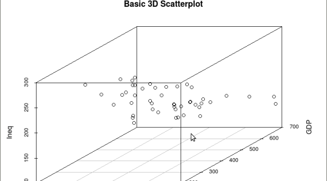
As is often the case in behavioral research we want to evaluate models that involve more than two variables. For multivariate models scatter plots can be generated using a 3 dimensional version of the R plot() function. For the above model we can add a third variable ‘Ineq’ from the dataset which is a measure the distribution of wealth in the population. Since we are now working with a multivariate linear model of the form ‘y = b1(x1) + b2(x2) + a’ we can use the R function scatterplot3d() to generate a 3 dimensional representation of the variables.

Once again we use the MASS package and the dataset  ‘UScrime’ for the graph data. The code is seen below:

####################################################
## create a 3d graph using the variables y, GDP, and Ineq
####################################################
#
library(scatterplot3d)   ##load scatterplot3d function
require(MASS)
attach(UScrime)   ## use data from UScrime dataset
scatterplot3d(y,GDP, Ineq,
main=”Basic 3D Scatterplot”) ## graph 3 variables, y
#
###################################################

The following graph is produced:

screenshot-graphics-device-number-2-active-%27rkward%27

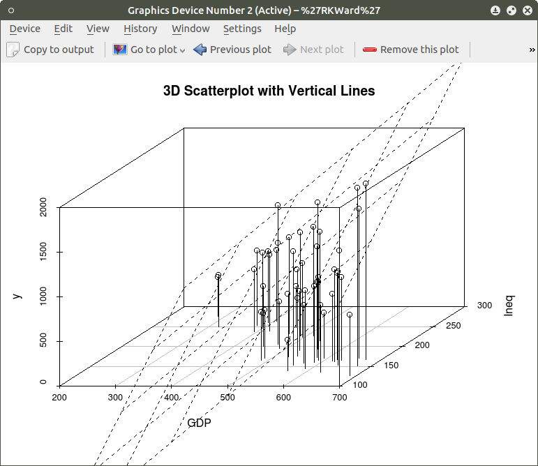
The above code will generate a basic 3d plot using default values. We can add straight lines from the plane of the graph to each of the data points by setting the graph type option as ‘type=”h”, as seen in the code below:

##############################################

require(MASS)
library(scatterplot3d)
attach(UScrime)
model <- scatterplot3d(GDP, Ineq, y,
type=”h”, ## add vertical lines from plane with this option
main=”3D Scatterplot with Vertical Lines”)
####################################################

This results in the graph:

screenshot-graphics-device-number-2-active-%27rkward%27-1

There are numerous options that can be used to go beyond the basic 3d plot. Refer to CRAN documentation to see these. A final addition to the 3d plot as discussed here is the code needed to generate the regression plane of our linear regression model using the y (crimerate), GDP, and Ineq variables. This is accomplished using the plane3d() option that will draw a plane through the data points of the existing plot. The code to do this is shown below:

##############################################
require(MASS)
library(scatterplot3d)
attach(UScrime)
model <- scatterplot3d(GDP, Ineq, y,
type=”h”,   ## add vertical line from plane to data points with this #option
main=”3D Scatterplot with Vertical Lines”)
## now calculate and add the linear regression data
model1 <- lm(y ~ GDP + Ineq)   #
model$plane3d(model1)   ## link the 3d scatterplot in ‘model’ to the ‘plane3d’ option with ‘model1’ regression information
#
####################################################

The resulting graph is:

screenshot-graphics-device-number-2-active-%27rkward%27-2

To draw a regression plane through the data points only change the ‘type’ option to ‘type=”p” to show the data points without vertical lines to the plane. There are also many other options that can be used. See the CRAN documentation to review them.

I have hopefully shown that relatively simple R code can be used to generate some informative and useful graphs. Once you start to become aware of how to use the multitude of options for these functions you can have virtually total control of the visual presentation of data. I will discuss some additional simple graphs in the next tutorial that I post.

R For Beginners: Some Simple R Code to do Common Statistical Procedures, Part Two


An R tutorial by D. M. Wiig

This posting contains an embedded Word document. To view the document full screen click on the icon in the lower right hand corner of the embedded document.


R For Beginners: Basic R Code for Common Statistical Procedures Part I


An R tutorial by D. M. Wiig

This section gives examples of code to perform some of the most common elementary statistical procedures. All code segments assume that the package ‘car’ has been loaded and the file ‘Freedman’ has been loaded as the active dataset. Use the menu from the R console to load the ’car’ dataset or use the following command line to access the CRAN site list and packages:


install.packages()

Once the ’car’ package has been downloaded and installed use the following command to make it the active library.

require(car)

Load the ‘Freedman’ data file from the dataset ‘car’

data(Freedman, package="car")

List basic descriptives of the variables:

summary(Freedman)

Perform a correlation between two variables using Pearson, Kendall or Spearman’s correlation:

cor(filename[,c("var1","var2")], use="complete.obs", method="pearson")

cor(filename[,c("var1","var2")], use="complete.obs", method="spearman")

cor(filename[,c("var1","var2")], use="complete.obs", method="kendall")

Example:

cor(Freedman[,c("crime","density")], use="complete.obs", method="pearson")

cor(Freedman[,c("crime","density")], use="complete.obs", method="kendall")

cor(Freedman[,c("crime","density")], use="complete.obs", method="spearman")

In the next post I will discuss basic code to produce multiple correlations and linear regression analysis.  See other tutorials on this blog for more R code examples for basic statistical analysis.


R Video Tutorial: Basic R Code to Load a Data File and Produce a Histogram


R For Beginners:  Some Simple R Code to Load a Data File and Produce a Histogram

A tutorial by D. M. Wiig

I have found that a good method for learning how to write R code is to examine complete code segments written to perform specific tasks and to modify these procedures to fit your specific needs. Trying to master R code in the abstract by reading a book or manual can be informative but is more often confusing.  Observing what various code segments do by observing the results allows you to learn with hands-on additions and modifications as needed for your purposes.

In this document I have included a short video tutorial that discusses  loading a dataset from the R library, examining the contents of the dataset and selecting one of the variables to examine using a basic histogram.  I have included an annotated code chunk of the procedures discussed in the video.

The video appears below with the code segment following.

Here is the annotated code used in the video:

###################################
#use the dataset mtcars from the ‘datasets’ package
#select the variable mpg to do a histogram
#show a frequency distribution of the scores
##########################################
#library is ‘datasets’
#########################################
library(“datasets”)
#########################################
#take a look at what is in ‘datasets’
#########################################
library(help=”datasets”)
#######################################
#take a look at the ‘mtcars’ data
#########################################
View(mtcars)
#######################################
#now do a basic histogram with the hist function
###########################################
hist(mtcars$mpg)
#############################################
#dress up the graph; not covered in the video but easy to do
############################################
hist(mtcars$mpg, col=”red”, xlab = “Miles per Gallon”, main = “Basic Histogram Using ‘mtcars’ Data”)
###################################################


R For Beginners: A Video Tutorial on Installing and Using the Deducer Statistics Package


R For Beginners:  A Video Tutorial on Installing and Using the Deducer Statistics Package with the R Console

In previous tutorials I have discussed the use of R Commander and Deducer statistical packages that provide a menu based GUI for R.  In this video tutorial I will discuss downloading and installing the Deducer statistics package.  This video is designed to support my previous tutorial on the same subject.

I have embedded the video below,   I hope you find this tutorial  a useful adjunct to installing and using the menu based Deducer package.

This document is an embedded Word document.  To view it full screen click on the icon in the lower right corner of the screen


R For Beginners: Installing the JGR GUI On a Linux Platform


A Tutorial by D. M. Wiig

This is an embedded Word document.  To view it full screen click on the icon in the lower right cornet of the document.

Watch for more tutorials discussing  R statistics on a Linux platform.

How to Install the Latest Version of R Statistics on Your Raspberry Pi


R for Beginners:  How to Install the Latest Version of R Statistics on Your Raspberry Pi

A tutorial by D. M. Wiig

One of the nice characteristics of open source software such as R is the rapid development of new releases and updates.  While the base core remains stable for a period of time there is a considerable amount of updating,  adding, and removing the component packages.  At the time of this writing the latest iteration is R version 3.3.1, “Bug in Your Hair.” If you are using a Windows platform you will likely go directly to the archive web site and download the latest distribution as a Windows executable installation package.

If you are using a Linux distribution  such as Ubuntu or Debian, the process of adding software is usually accomplished via the menu based installer.  These software installers allow  R and its dependencies to be downloaded from the community archive.

One of the disadvantages of using this approach is that the versions of some software in the community archives may not be updated to the latest version.  This is often the case with R as well as with many other software packages.

To insure that you are downloading the latest R version you need to use the platform’s command line to install what is needed.  You can add the URL’s of some backport archives that are more likely to be kept up to date with current releases.  As an example In this tutorial I will use the R statistical software that I am running on my Raspberry Pi 3 board with a Raspbian OS and the new PIXEL desktop.

Regardless of which Linux distribution you are using first open a command console from the desktop menu. Make sure all is up to date by using the command:

pi@raspberrypi:~ $ sudo apt-get update
This will insure all appropriate packages currently installed are running the latest updates.  If you are running a Raspbian distribution such as jessie you will need to edit the /etc/apt/sources.list file to add a backport to the latest version of R.  Start the nano editor by using the command:

sudo nano /etc/apt/sources.list

This should produce the output as seen below:

pi@raspberrypi:~ $ sudo nano /etc/apt/sources.list

------------------------------------------------
GNU nano 2.2.6 File: /etc/apt/sources.list

deb http://mirrordirector.raspbian.org/raspbian/ jessie main contrib non-free r$
# Uncomment line below then 'apt-get update' to enable 'apt-get source'
deb-src http://archive.raspbian.org/raspbian/ jessie main contrib non-free rpi
deb http://archive.raspbian.org/raspbian/ stretch main
deb http://mirror.las.iastate.edu/CRAN/bin/linux/debian/ jessie main
deb http://mirror.las.iastate.edu/CRAN/bin/linux/ubuntu xenial/

[ Read 8 lines ]
^G Get Help ^O WriteOut ^R Read File ^Y Prev Page ^K Cut Text ^C Cur Pos
^X Exit ^J Justify ^W Where Is ^V Next Page ^U UnCut Text^T To Spell

As is seen above there are several lines containing the standard  Raspbian archives to search.


If you are using a Debian distribution you would add the following line to the file:

http://mirror.las.iastate.edu/CRAN/bin/linux/debian/ jessie main

Replace the 'jessie' portion with the name of the specific Debian distribution you are using replace the 'mirror' portion with the R CRAN mirror that you use.  You also need to add the line that provides the URL of a Raspian 'stretch' archive that contains the most recent updates of many different software packages.  In my case I was looking for the latest R release, but you should search this this archive for the latest version of any software package you are installing.

If you are using an Ubuntu distribution add a line with the appropriate changes for the specific Ubuntu distribution that you are using. 
Check with the documentation provided with your specific Linux distribution to see if there is also a 'stretch' archive maintained for new versions. 

Once these changes are made exit the nano editor using the ^O key command to write the file and then the ^X key command to return to the command line.  You should now be able to issue the command:

pi@raspberrypi:~ $ sudo apt-get install r-base r-base-core r-base-dev

Once the download and install processes have completed you should now be able to invoke R from the command line or menu and see the latest version:

pi@raspberrypi:~ $ R

R version 3.3.2 RC (2016-10-23 r71578) -- "Sincere Pumpkin Patch"
Copyright (C) 2016 The R Foundation for Statistical Computing
Platform: arm-unknown-linux-gnueabihf (32-bit)

R is free software and comes with ABSOLUTELY NO WARRANTY.
You are welcome to redistribute it under certain conditions.
Type 'license()' or 'licence()' for distribution details.

 Natural language support but running in an English locale

R is a collaborative project with many contributors.
Type 'contributors()' for more information and
'citation()' on how to cite R or R packages in publications.

Type 'demo()' for some demos, 'help()' for on-line help, or
'help.start()' for an HTML browser interface to help.
Type 'q()' to quit R.

> 


For other Linux distributions you would add a line similar to the above examples in the /etc/apt/sources.list. Check the documentation for your specific Linux platform for further information about backport archives.

R For Beginners: Installing the latest version of R on a Linux platform


R for Beginners:  Installing the latest version of R on a Linux platform

A tutorial by D. M. Wiig

One of the nice characteristics of open source software such as R is the rapid development of new releases and updates.  While the base core remains stable for a period of time there is a considerable amount of updating,  adding, and removing the component packages.  At the time of this writing the latest iteration is R version 3.3.1, “Bug in Your Hair.” If you are using a Windows platform you will likely go directly to the archive web site and download the latest distribution as a Windows executable installation package.

If you are using a Linux distribution  such as Ubuntu or Debian, the process of adding software is usually accomplished via the menu based installer.  These software installers allow  R and its dependencies to be downloaded from the community archive.

One of the disadvantages of using this approach is that the versions of some software in the archives may not be updated to the latest version.  This is often the case with R.

To insure that you are downloading the latest R version you need to use the platform’s command line to install what is needed.  Regradless of which Linux distribution you are using first open a command console from the desktop menu. Make sure all is up to date by using the command:

pi@raspberrypi:~ $ sudo apt-get update
This will insure all appropriate packages currently installed are running the latest updates.  If you are running a Debian distribution such as jessie you will need to edit the /etc/apt/sources.list file to add a backport to the latest version of R.  Use the nano editor by using the command:

sudo nano /etc/apt/sources.list

This should produce the output as seen below:

pi@raspberrypi:~ $ sudo nano /etc/apt/sources.list

------------------------------------------------
GNU nano 2.2.6 File: /etc/apt/sources.list

deb http://mirrordirector.raspbian.org/raspbian/ jessie main contrib non-free r$
# Uncomment line below then 'apt-get update' to enable 'apt-get source'
deb-src http://archive.raspbian.org/raspbian/ jessie main contrib non-free rpi
deb http://archive.raspbian.org/raspbian/ stretch main
deb http://mirror.las.iastate.edu/CRAN/bin/linux/debian/ jessie main
deb http://mirror.las.iastate.edu/CRAN/bin/linux/ubuntu xenial/

[ Read 8 lines ]
^G Get Help ^O WriteOut ^R Read File ^Y Prev Page ^K Cut Text ^C Cur Pos
^X Exit ^J Justify ^W Where Is ^V Next Page ^U UnCut Text^T To Spell


If you are using a Debian distribution you would add the line to the file

http://mirror.las.iastate.edu/CRAN/bin/linux/debian/ jessie main

Replace the mirror portion with <URL of your favorite CRAN mirror>.  Replace the 'jessie' portion with the name of the specific Debian distribution you are using.

If you are using an Ubuntu distribution add a line with the appropriate changes for the specific Ubuntu distribution that you are using.

Once these changes are made exit the nano editor using the ^O key command to write the file and then the ^X key command to return to the command line.  You should now be able to issue the command:

pi@raspberrypi:~ $ sudo apt-get install r-base r-base-core r-base-dev

Once the download and install processes have completed you should now be able to invoke R from the command line or menu and see the latest version:

pi@raspberrypi:~ $ R

R version 3.3.2 RC (2016-10-23 r71578) -- "Sincere Pumpkin Patch"
Copyright (C) 2016 The R Foundation for Statistical Computing
Platform: arm-unknown-linux-gnueabihf (32-bit)

R is free software and comes with ABSOLUTELY NO WARRANTY.
You are welcome to redistribute it under certain conditions.
Type 'license()' or 'licence()' for distribution details.

 Natural language support but running in an English locale

R is a collaborative project with many contributors.
Type 'contributors()' for more information and
'citation()' on how to cite R or R packages in publications.

Type 'demo()' for some demos, 'help()' for on-line help, or
'help.start()' for an HTML browser interface to help.
Type 'q()' to quit R.

> 


For other Linux distributions you would add a line similar to the above examples in the /etc/apt/sources.list. Check the documentation for your specific Linux platform for further information.


R Video Tutorial For Beginners: Installing And Using the Rcommander GUI


R Video Tutorial For Beginners: Installing And Using the Rcommander GUI

A tutorial video by D. M. Wiig

In my recent series of tutorials for those interested in the R statistical programming language I have discussed both the installation and use of the R console and R Commander statistics GUI.  Before viewing the tutorial make sure the R Commander package has been download into your R library via the Install Packages menu option.  This procedure was discussed in the previously posted R Commander tutorial.

Relative to this first tutorial I have have created a video that covers the initial installation of R Commander.  The video is seen below:

Click the icon in the lower right side of the screen to view the tutorial in full screen mode.

I hope that you find this useful in your pursuit of learning about  R statistics.

R for beginners: Installing Deducer in the R Windows GUI


R for beginners: Installing Deducer in the R Windows GUI

A tutorial by D.M. Wiig

This is posted as a Word document.  To view the post full screen click on the button in the lower right corner of this window.

More on this topic to be posted soon!

Resources and Information About R Statistics and Programming