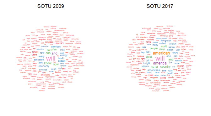
In part one of this tutorial, I discussed the use of the tm and wordcloud packages to create a visual representation of the most frequently used words in the 2026 Presidential State of the Union Address. I also discussed the code needed to generate an initial analysis of the wordcloud with a list of the 15 most used words and their frequency. I also discussed code that calculated a matrix consisting of the relative strength of association among 10 most commonly used words and other words used in the address. In this tutorial I will present code to display two wordclouds, one containing frequently used words in the 2009 State of the Union Address, and one containing the frequently used words from the 2017 State of the Union Address. I will also show the R code necessary to produce a simple bar graph of the most frequently used words and the association matrix for each wordcloud.

The required R code is essentially the same as the code used in part one of the tutorial with additional code to create the second wordcloud and associated statistics and to display the graphics side by side. I have also included a simple bar graph to display a comparison of the most frequently used words in each SOTU. As is my practice in all of my tutorials I have included a running commentary for each major section of the code. Make sure that you make the appropriate changes in your path to the SOTU files to be loaded before running the program and that all required packages are installed in your R libraries. As always, make sure that you are running up to date R-base and RStudio versions.

###################################################
#wordcloudcomp, displays sotu09 and sotu17 side by side
#calculates word counts, most frequent words, word assoc #strengths
###################################################
###################################################
#Load required packages
###################################################
install.packages(“tm”) #processes data
install.packages(“wordcloud”) #creates visual plot
install.packages(“tidyverse”) #graphics utilities
install.packages(“readr”) #to load text files
install.packages(“RColorBrewer”) #for color graphics
install.packages(“ggplot2”)
###################################################
#Read in text file for 2009 SOTU
library(readr)
statu09 <- read_table(“E:/dellfiles/statu09.txt”, col_names = FALSE)
#read in text file for 2017 SOTU
statu17 <- read_table(“E:/dellfiles/statu17.txt”, col_names = FALSE)
###################################################
#convert each text to Corpus format
#docs09 <- statu09 2009 address
#docs17 <- statu17 2017 address
###################################################
library(tm)
docs09 <- Corpus(VectorSource(statu09))
#
docs17 <- Corpus(VectorSource(statu17))
#
###################################################
#clean each file; remove punctuation, stop words, white space
#use either “en” or “SMART” predefined set for stop words #removal
###################################################
library(tm)
library(wordcloud)
#
data(docs09)
docs09 <- tm_map(docs09, function(x)removeWords(x,stopwords(“en”)))
docs09 <- tm_map(docs09,removePunctuation) #remove punctuation
docs09 <- tm_map(docs09,stripWhitespace) #remove white space
#
data(docs17)
docs17 <- tm_map(docs17,function(x)removeWords(x,stopwords(“en”)))
docs17 <- tm_map(docs17,removePunctuation) #remove punctuation
docs17 <- tm_map(docs17,stripWhitespace) #remove white space
#
###################################################
#Cleaned corpus is now formatted into text document matrix
#Then frequency count done for each word in matrix
#dmat <-create matrix; dval <-sort; dframe <-count word frequencies
###################################################
#2009 address
#
docmat09 <- TermDocumentMatrix(docs09)
dmat09 <- as.matrix(docmat09)
dval09 <- sort(rowSums(dmat09),decreasing=TRUE)
dframe09 <- data.frame(word=names(dval09),freq=dval09)
#
#2017 address
docmat17 <- TermDocumentMatrix(docs17)
dmat17 <- as.matrix(docmat17)
dval17 <- sort(rowSums(dmat17),decreasing=TRUE)
dframe17 <- data.frame(word=names(dval17),freq=dval17)
#
###################################################
#create 2 panels, each to display a wordcloud
###################################################
#
par(mfrow=c(1,2))
#
####################################################create 2009 wordcloud
###################################################
#
library(RColorBrewer)
set.seed(1234) #use if random.color=TRUE
par(bg=”white”) #background color
wordcloud(dframe09$word,dframe09$freq,colors=brewer.pal(8,”Set1″),random.order=FALSE,scale=c(2,0.35),min.freq=2,max.words=200,rot.per=0.0)
# Add a title above the plot
mtext(“SOTU 2009″, side = 3, line = 2, cex = 1.5)
#
###################################################
#create 2017 wordcloud
###################################################
#
library(RColorBrewer)
set.seed(1234) #use if random.color=TRUE
par(bg=”yellow”) #background color
wordcloud(dframe17$word,dframe17$freq,colors=brewer.pal(8,”Set1″),random.order=FALSE,scale=c(2,0.35),min.freq=2,max.words=200,rot.per=0.0)
# Add a title above the plot
mtext(“SOTU 2017”, side = 3, line = 2, cex = 1.5)
#
###################################################
#this section contains code for printing word freq tables;
#doing bar graphs of word freq; word assoc analysis;
#code to print 15 most used words with freq;
#capture output in form to copy to Tex or other editor
###################################################
#for 2017 address
out <- capture.output(head(dframe17,15))
writeLines(out)
#
###################################################
#for 2009 address
out <- capture.output(head(dframe17,15))
writeLines(out)
#
####################################################code to print simple bar graph of most frequently
#used words for each SOTU; set to show 15 words
###################################################
#for 2009 address
library(ggplot2)
#
barplot(dframe09[1:15,]$freq, las=2, names.arg = dframe09[1:15,]$word, col = “blue”)
# Add a title above the plot
mtext(“SOTU 2009 Word Frequency”, side = 3, line = 2, cex = 1.5)
#
###################################################
#for 2017 address
library(ggplot2)
#
barplot(dframe17[1:15,]$freq, las=2, names.arg = dframe17[1:15,]$word, col = “red”)
# Add a title above the plot
mtext(“SOTU 2017 Word Frequency”, side = 3, line = 2, cex = 1.5)
#
###################################################
#code to find associations among specified terms
#drops cor < .25
#initial setup for most frequent words; 10 most frequently used
###################################################
#for 2009 address
out <- capture.output((findAssocs(docmat09,terms = c(“and”,”will”,”know”,”economy”,”every”,”now”,”can”,”plan”,”but”,”economy”),corlimit = .25)))
writeLines(out)
#
#for 2017 address
out <- capture.output((findAssocs(docmat17,terms = c(“and”,”will”,”america”,”american”,”must”,”country”,”new”,”people”,”great”,”world”),corlimit = .25)))
writeLines(out)
#
######################################################################################################

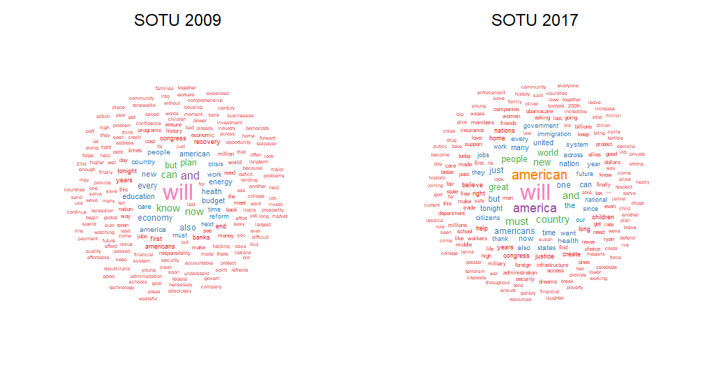
The wordclouds are seen side by side below.

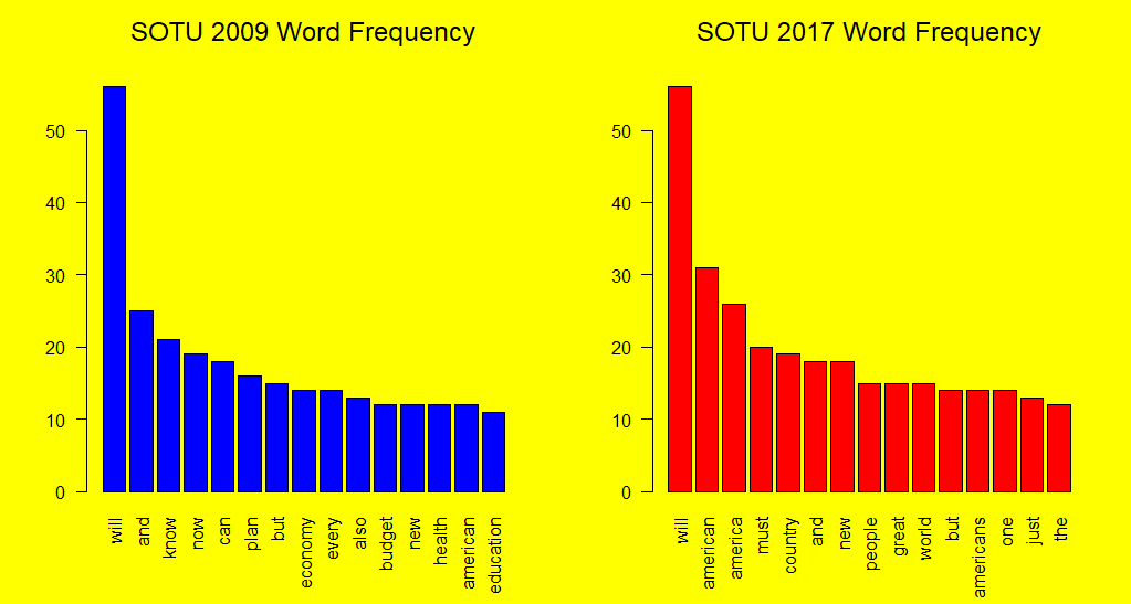
The bar graph that follows show the frequencies for the most used words in each address.

In order to save space, I have uploaded the word association matrix data for each SOTU into a markdown file that can be viewed by clicking the link at the bottom of this posting.

In parts one and two of this tutorial I focused on an approach that treats the document as a matrix of meaningful individual words. This approach is a good starting point. I will cap this approach in part three by discussing two additional wordcloud functions, the comparison.cloud and the commonality.cloud functions. In part four of this tutorial, I will present code that will allow analysis of the sentences and structure of the entire document. This will allow the use of a more advanced R package for text analysis, the contentanalysis  package.

This document .pdf click -> sotu0917

Word association matrix click ->0917assoctab

All R programming for this project was done using RStudio 2026.07.0+139 “Pacific Dogwood.”
This PDF document was produced using TeXstudio 4.9.5 (git 4.9.5)
Using Qt Version 6.11.0, compiled with Qt 6.11.0 R.
R, RStudio, and TeXstudio are free, open-source software.