Tag Archives: using r for statistics

R Tutorial: A Simple Script to Create and Analyze a Data File, Part Two


A simple R script to create and analyze a data file:part two:    A tutorial by D.M. Wiig

In part one I discussed creating a simple data file containing the height and weight of 10 subjects.  In part two I will discuss the script needed to create a simple scatter diagram of the data and perform a basic Pearson correlation.  Before attempting to continue the script in this tutorial make sure that you have created and save the data file as discussed in part one.

To conduct a correlation/regression analysis of the data we want to first view a simple scatter plot. Load a library named ‘car’ into R memory. Use the command:

> library(car)

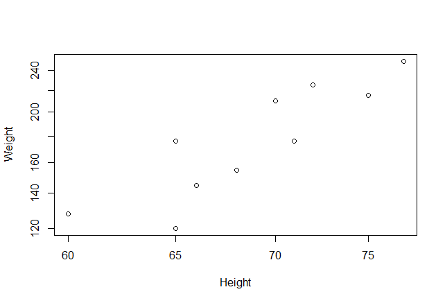
Then issue the following command to plot the graph:

> plot(Height~Weight, log=”xy”, data=Sampledatafile)

The output is seen below:
scatter1

We can calculate a Pearson’s Product Moment correlation coefficient by using the command:

> # Pearson rank-order correlations between height and weight

> cor(Sampledatafile[,c(“Height”,”Weight”)], use=”complete.obs”, method=”pearson”)

Which results in:

Height Weight

Height 1.0000000 0.8813799

Weight 0.8813799 1.0000000

To run a simple linear regression for Height and Weight use the following code. Note that the dependent variable (Weight) is listed firt:

> model <-lm(Weight~Height, data=Sampledatafile)

> summary(model)

Call:

lm(formula = Weight ~ Height, data = Sampledatafile)

Residuals:

Min 1Q Median 3Q Max

-30.6800 -16.9749 -0.8774 19.9982 25.3200

Coefficients:

Estimate Std. Error t value Pr(>|t|)

(Intercept) -337.986 98.403 -3.435 0.008893 **

Height 7.518 1.425 5.277 0.000749 ***

Signif. codes: 0 ‘***’ 0.001 ‘**’ 0.01 ‘*’ 0.05 ‘.’ 0.1 ‘ ’ 1

Residual standard error: 21.93 on 8 degrees of freedom

Multiple R-squared: 0.7768, Adjusted R-squared: 0.7489

F-statistic: 27.85 on 1 and 8 DF, p-value: 0.0007489

>

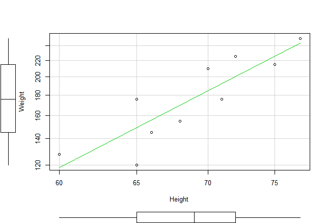
To plot a regression line on the scatter diagram use the following command line. Note that we enter the y (dependent)variable first and then the x (independent)variable:

> scatterplot(Weight~Height, log=”xy”, reg.line=lm, smooth=FALSE, spread=FALSE,

+ data=Sampledatafile)

>

This will produce a graph as seen below. Note that box plots have also been included in the output:
scatter2

This tutorial has hopefully demonstrated that complex tasks can be accomplished with relatively simple command line script. I will explore more of these simple scripts in future tutorials.

More to Come:


R Tutorial: A Script to Create and Analyze a Simple Data File, Part One


R Tutorial: A Simple Script to Create and Analyze a Data File, Part One

By D.M. Wiig

In this tutorial I will walk you through a simple script that will show you how to create a data file and perform some simple statistical procedures on the file. I will break the code into segments and discuss what each segment does. Before starting this tutorial make sure you have a terminal window open and open R from the command line.

The first task is to create a simple data file. Let’s assume that we have some data from 10 individuals measuring each person’s height and weight. The data is shown below:

Height(inches) Weight(lbs)

72               225

60               128

65               176

75               215

66               145

65               120

70               210

71               176

68               155

77               250

We can enter the data into a data matrix by invoking the data editor and entering the values. Please note that the lines of code preceded by a # are comments and are ignored by R:

#Create a new file and invoke the data editor to enter data

#Create the file Sampledatafile, height and weight of 10 s subjects

Sampledatafile <-data.frame()

Sampledatafile <-edit(Sampledatafile)

You will see a window open that is the R Data Editor. Click on the column heading ‘var1’ and you will see several different data types in the drop down menu. Choose the ‘real’ data type. Follow the same procedure to set the data type for the second column. Enter the data pairs in the columns, with height in the first column and weight in the second column. When the data have been entered click on the var1 heading for column 1 and click ‘Change Name.’ Enter ‘Height’ to label the first column. Follow the same steps to rename the second column ‘Weight.’

Once both columns of data have been entered you can click ‘Quit.’ The datafile ‘Sampledatafile’ is now loaded into memory.

To run so me basic descriptive statistics use the following code:

> #Run descriptives on the data

> summary(Sampledatafile)

The output from this code will be:

  Height                Weight

Min. :60.00          Min. :120.0

1st Qu.:65.25        1st Qu.:147.5

Median :69.00        Median :176.0

Mean :68.90          Mean :180.0

3rd Qu.:71.75        3rd Qu.:213.8

Max. :77.00          Max. :250.0

>

To view the data file use the following lines of code:

>#print the datafile ‘Sampledatafile’ on the screen

> print(Sampledatafile)

You will see the output:

Height          Weight

1 72             225

2 60             128

3 65             176

4 75             215

5 66             145

6 65             120

7 70             210

8 71             176

9 68             155

10 77            250

In Part Two I will discuss an R script to do a simple correlation and scatter diagram.  Check back later!