Visual Representation of Text Data Sets Using the R tm and wordcloud Packages: Part One
Douglas M. Wiig
This paper is the next installment in series that examines the use of R scripts to present and analyze complex data sets using various types of visual representations. Previous papers have discussed data sets containing a small number of cases and many variable, and data sets with a large number of cases and many variables. The previous tutorials have focused on data sets that were numeric. In this tutorial I will discuss some uses of the R packages tm and wordcloud to meaningfully display and analyze data sets that are composed of text. These types of data sets include formal addresses, speeches, web site content, Twitter posts, and many other forms of text based communication.
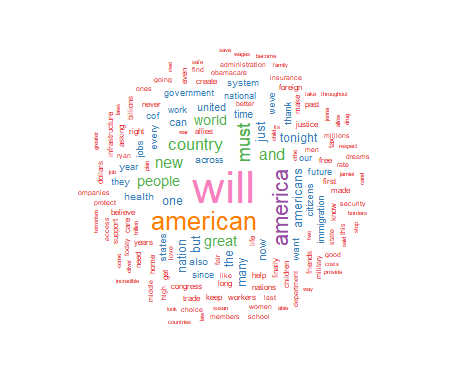
I will present basic R script to process a text file and display the frequency of significant words contained in the text. The results include a visual display of the words using the size of the font to indicate the relative frequency of the word. This approach displays increasing font size as specific word frequency increases. This type of visualization of data is generally referred to as a "wordcloud." To illustrate the use of this approach I will produce a wordcloud that contains the text from the 2017 Presidental State of the Union Address.
There are generally four steps involved in creating a wordcloud. The first step involves loading the selected text file and required packages into the R environment. In the second step the text file is converted into a corpus file type and is cleaned of unwanted text, punctuation and other non-text characters. The third step involves processing the cleaned file to determine word frequencies, and in the fourth step the wordcloud graphic is created and displayed.
Installing Required Packages
As discussed in previous tutorials I would highly recommend the use of an IDE such as RStudio when composing R scripts. While it is possible to use the basic editor and package loader that is part of the R distribution, an IDE will give you a wealth of tools for entering, editing, running, and debugging script. While using RStudio to its fullest potential has a fairly steep learning curve, it is relatively easy to successfully navigate and produce less complex R projects such as this one.
Before moving to the specific code for this project run a list of all of the packages that are loaded when R is started. If you are using RStudio click on the "Packages" tab in the lower right quadrant of the screen and look through the list of packages. If you are using the basic R script editor and package loader, at the command prompt use the following command:
#####################################################################################
>installed.packages()
#####################################################################################
The command produces a list of all currently installed packages. Depending on the specific R version that you are using the packages for this project may or may not be loaded and available. I will assume that they will need to be installed. The packages to be loaded are tm, wordcloud, tidyverse, readr, and RColorBrewer. Use the following code:
#############################################################################
#Load required packages
#############################################################################
install.packages("tm") #processes data
install.packages("wordcloud") #creates visual plot
install.packages("tidyverse") #graphics utilities
install.packages("readr") #to load text files
install.packages("RColorBrewer") #for color graphics
#############################################################################
Once the packages are installed the raw text file can be loaded. The complete text of Presidential State of the Union Addresses can be readily accessed on the government web site https://www.govinfo.gov/features/state-of-the-union. The site has sets of complete text for various years that can be downloaded in several formats. For this project I used the 2017 State of the Union downloaded in text format. To load and view the raw text file in the R environment use the "Import Dataset" tab in the upper right quadrant of RStudio or the code below:
#############################################################################
library(readr)
yourdatasetname <- read_table2("path to your data file", col_names = FALSE)
View(dataset)
#############################################################################
Processing The Data
The goal of this step is to produce the word frequencies that will be used by wordcloud to create the wordcloud graphic display. This process entails converting the raw text file into a corpus format, cleaning the file of unwanted text, converting the cleaned file to a text matrix format, and producing the word frequency counts to be graphed. The code below accomplishes these tasks. Follow the comments for a description of each step involved.
###########################################################################
#Take raw text file statu17 and convert to corpus format named docs17
###########################################################################
library(tm)
docs17 <- Corpus(VectorSource(statu17))
###########################################################################
###########################################################################
#Clean punctuation, stopwords, white space
#Three passes create corpus vector source from original file
#A corpus is a collection of text
###########################################################################
library(tm)
library(wordcloud)
data(docs17)
docs17 <- tm_map(docs17,removePunctuation) #remove punctuation
docs17 <- tm_map(docs17,removeWords,stopwords("english")) #remove stopwords
docs17 <- tm_map(docs17,stripWhitespace) #remove white space
###########################################################################
#Cleaned corpus is now formatted into text document matrix
#Then frequency count done for each word in matrix
#dmat <-create matrix; dval <-sort; dframe <-count word frequencies
#docmat <- converts cleaned corpus to text matrix for processing
###########################################################################
docmat <- TermDocumentMatrix(docs17)
dmat <- as.matrix(docmat)
dval <- sort(rowSums(dmat),decreasing=TRUE)
dframe <- data.frame(word=names(dval),freq=dval)
###########################################################################
Once these steps have been completed the data frame "dframe" will now be used by the wordcloud package to produce the graphic.
Producing the Wordcloud Graphic
We are now ready to produce the graphic plot of word frequencies. The resulting display can be manipulated using a number of settings including color schemes, number of words displayed, size of the wordcloud, minimum word frequency of words to display, and many other factors. Refer to Appendix B for additional information.
For this project I have chosen to use a white background and a multi-colored word display. The display is medium size, with 150 words maximum, and a minimum word frequency of two. The resulting graphic is shown in Figure 1. Use the code below to produce and display the wordcloud:
##########################################################################################
#Final step is to use wordcloud to generate graphics
#There are a number of options that can be set
#See Appendix for details
#Use RColorBrewer to generate a color wordcloud
#RColorBrewer has many options, see Appendix for details
##########################################################################################
library(RColorBrewer)
set.seed(1234) #use if random.color=TRUE
par(bg="white") #background color
wordcloud(dframe$word,dframe$freq,colors=brewer.pal(8,"Set1"),random.order=FALSE,
scale=c(2.75,0.20),min.freq=2,max.words=150,rot.per=0.35)
##########################################################################################
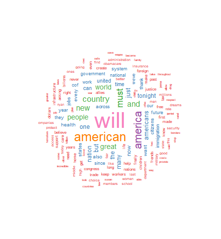 As seen above, the wordcloud display is arranged in a manner with the most frequently used words in the largest font at the center of the graph. As word frequency drops there are somewhat concentric rings of words in smaller and smaller fonts with the smallest font outer rings set by the wordcloud parameter min.freq=2. At this point I will leave an analysis of the wordcloud to the interpretation of the reader.
In part two of this tutorial I will discuss further use of the wordcloud package to produce comparison wordclouds using SOTU text files from 2017, 2018, 2019, and 2020. I will also introduce part three of the tutorial which will discuss using wordcloud with very large text data sets such as Twitter posts.
Appendix A: Resources and References
This section contains links and references to resources used in this project. For further information on specific R packages see the links below.
Package tm:
https://cran.r-project.org/web/packages/tm/tm.pdf
Package RColorBrewer:
https://cran.r-project.org/web/packages/RColorBrewer/RColorBrewer.pdf
Package readr:
https://cran.r-project.org/web/packages/readr/readr.pdf
Package wordcloud:
https://cran.r-project.org/web/packages/wordcloud/wordcloud.pdf
Package tidyverse
https://cran.r-project.org/web/packages/tidyverse/tidyverse.pdf
To download the RStudio IDE:
https://www.rstudio.com/products/rstudio/download
General works relating to R programming:
Robert Kabacoff, R in Action: Data Analysis and Graphics With R, Sheleter Island, NY: Manning Publications, 2011.
N.D. Lewis, Visualizing Complex Data in R, N.D. Lewis, 2013.
The text data for the 2017 State of the Union Address was downloaded from:
https://www.govinfo.gov/features/state-of-the-union
Appendix B: R Functions Syntax Usage
This appendix contains the syntax usage for the main R functions used in this paper. See the links in Appendix A for more detail on each function.
readr:
read_table2(file,col_names = TRUE,col_types = NULL,locale = default_locale(),na = "NA",
skip = 0,n_max = Inf,guess_max = min(n_max, 1000),progress = show_progress(),comment = "",
skip_empty_rows = TRUE)
wordcloud:
wordcloud(words,freq,scale=c(4,.5),min.freq=3,max.words=Inf,
random.order=TRUE, random.color=FALSE, rot.per=.1,
colors="black",ordered.colors=FALSE,use.r.layout=FALSE,
fixed.asp=TRUE, ...)
rcolorbrewer:
brewer.pal(n, name)
display.brewer.pal(n, name)
display.brewer.all(n=NULL, type="all", select=NULL, exact.n=TRUE,colorblindFriendly=FALSE)
brewer.pal.info
tm:
tm_map(x, FUN, ...)
All R programming for this project was done using RStudio Version 1.2.5033
The PDF version of this document was produced using TeXstudio 2.12.6
Author: Douglas M. Wiig 4/01/2021
Web Site: http://dmwiig.net
Click the links below to open the PDF version of this post.
As seen above, the wordcloud display is arranged in a manner with the most frequently used words in the largest font at the center of the graph. As word frequency drops there are somewhat concentric rings of words in smaller and smaller fonts with the smallest font outer rings set by the wordcloud parameter min.freq=2. At this point I will leave an analysis of the wordcloud to the interpretation of the reader.
In part two of this tutorial I will discuss further use of the wordcloud package to produce comparison wordclouds using SOTU text files from 2017, 2018, 2019, and 2020. I will also introduce part three of the tutorial which will discuss using wordcloud with very large text data sets such as Twitter posts.
Appendix A: Resources and References
This section contains links and references to resources used in this project. For further information on specific R packages see the links below.
Package tm:
https://cran.r-project.org/web/packages/tm/tm.pdf
Package RColorBrewer:
https://cran.r-project.org/web/packages/RColorBrewer/RColorBrewer.pdf
Package readr:
https://cran.r-project.org/web/packages/readr/readr.pdf
Package wordcloud:
https://cran.r-project.org/web/packages/wordcloud/wordcloud.pdf
Package tidyverse
https://cran.r-project.org/web/packages/tidyverse/tidyverse.pdf
To download the RStudio IDE:
https://www.rstudio.com/products/rstudio/download
General works relating to R programming:
Robert Kabacoff, R in Action: Data Analysis and Graphics With R, Sheleter Island, NY: Manning Publications, 2011.
N.D. Lewis, Visualizing Complex Data in R, N.D. Lewis, 2013.
The text data for the 2017 State of the Union Address was downloaded from:
https://www.govinfo.gov/features/state-of-the-union
Appendix B: R Functions Syntax Usage
This appendix contains the syntax usage for the main R functions used in this paper. See the links in Appendix A for more detail on each function.
readr:
read_table2(file,col_names = TRUE,col_types = NULL,locale = default_locale(),na = "NA",
skip = 0,n_max = Inf,guess_max = min(n_max, 1000),progress = show_progress(),comment = "",
skip_empty_rows = TRUE)
wordcloud:
wordcloud(words,freq,scale=c(4,.5),min.freq=3,max.words=Inf,
random.order=TRUE, random.color=FALSE, rot.per=.1,
colors="black",ordered.colors=FALSE,use.r.layout=FALSE,
fixed.asp=TRUE, ...)
rcolorbrewer:
brewer.pal(n, name)
display.brewer.pal(n, name)
display.brewer.all(n=NULL, type="all", select=NULL, exact.n=TRUE,colorblindFriendly=FALSE)
brewer.pal.info
tm:
tm_map(x, FUN, ...)
All R programming for this project was done using RStudio Version 1.2.5033
The PDF version of this document was produced using TeXstudio 2.12.6
Author: Douglas M. Wiig 4/01/2021
Web Site: http://dmwiig.net
Click the links below to open the PDF version of this post.
Tag Archives: programming
Book Review: Mastering Beaglebone Robotics
Richard Grimmett. Mastering Beaglebone Robotics. Birmingham, UK: Packt Publishing Ltd., 2014. ISBN #978-1-78398-890-7 http://bit.ly/MBbR8907
Book Review by Douglas M. Wiig
With the release of the Raspberry Pi single board computer a new generation of single board multi-platform and multi-use computers has rapidly developed. One of the newer boards to be developed is the Beaglebone Black which is a low cost, multi-functional package that has a number of core functionalities that facilitate building robotic projects. Grimmett’s Mastering Beaglebone Robotics is a very informative and readable guide to the development and implementation of several such projects. The finished projects are sophisticated, functional and educational. They also lend themselves to expansion into even more complex applications if the reader is so inclined.
This book is not intended for beginners with single board computing platforms or robotics but the author does go through the basics of setting up the Beaglebone and installing the necessary software to accommodate the projects in the book. If you are not yet comfortable with installing and configuring hardware and software or working with the Linux command line you should have a basic reference handy as you work through the initial hardware and software setup in chapter one of the book. The author does provide numerous photos and screen shots to help with the process. The author also uses very clear indications of how and what command line actions are used in installing and configuring various programs needed to set up the Beaglebone for the projects in the book.
Once the basic hardware and software are installed and running the author begins a discussion of robotics by taking the reader through a step by step process to create a movable project based on two tank tracks. The chapter covers the basics of using a motor and controller to power the project, the development and use of programs to control the vehicle and the use of voice commands to control the vehicle.
The author provides a detailed description along with numerous photos showing the build as it progresses. In the sections of the chapter where Beaglebone programming is covered the author uses very clear descriptions of the code that make the process easy to follow. Another nice feature of this book as well as other technical books in the Packt library is the availability for download of all of the code used in the book. This is a very handy feature and helps to prevent the frustration of coding errors that are inherent in entering the code from scratch on a keyboard. It also facilitates the debugging phase of the projects.
Once the basic mobile project platform is functional the author devotes two additional chapters to adding sensors of various kinds such as distance object detection, and adding vision and vision processing capabilities. Once again, the author uses numerous detailed photos, screen shots and programming detail in discussing these phases of the project. By the time the reader finishes chapter four of the book a fully functional, programmable movable platform has been developed.
Subsequent chapters of the book are devoted to additional projects that incorporate the basic principles of robotics learned in the initial project. The author discusses building robots that can walk, sail, and use GPS for navigation. There is also a discussion of a project robot that can be submerged and controlled remotely while under water.
The final two chapters of the book detail a quadcopter that is remotely controlled and an autonomous quadcopter that features programmed flight controlled by GPS. I found these chapters particularly interesting as one of my hobbies is flying radio controlled aircraft of various types. These two projects are rather advanced in nature and are more for readers interested in contributing to the development of such projects. In both projects the Beaglebone is used for higher level function such as GPS navigation, path planning and communications. Most of the low level functioning such as controlling the servo motors and other mechanical functions is accomplished by programming and incorporating a separate flight controller board.
As I mentioned earlier, one of the handy features of this book as well as others offered by Packt Publishing is the availability of the computer code used in each chapter of the book. The code used in Mastering Beaglebone Robotics is written in Python and there are files for each of the chapters (with the exception of chapters one and six). This is a useful feature not only for debugging purposes but for those readers who wish to develop other projects or add to the projects detailed in the book.
I found Mastering Beaglebone Robotics to be a good read and a readily usable guide to some of the more complex robotics concepts and construction practices. As indicated earlier this would not be a first book for one starting in either robotics or single-board computing platforms. For the reader with some experience in programming and construction practices the book is an interesting and informative source of information about a rapidly growing field in computer science technology and robotics.
——————————————————————
